Diffusion Models - III: Language Models
Can You Add Noise to a Word?

Introduction
In earlier posts, I talked about theory behind diffusion, did simple visual explorations to understand the mechanism better, learned about stable diffusion, and fine-tuned stable diffusion using LoRA for generating images in the style of vintage scientific engravings. We ended Part II with a question:
what happens when you try to diffuse something discrete?
Diffusion models generate images by adding Gaussian noise and learning to reverse it. The mathematics is beautiful and the results are spectacular. But images are continuous — each pixel is a real number, and you can add a little noise to a real number and still have a real number. Language is not like this. A sentence is a sequence of discrete tokens drawn from a finite vocabulary. You cannot add a small amount of Gaussian noise to the word “cat” and get a slightly noisy word. The word “cat” is either “cat” or it isn’t. The smooth, continuous machinery of Parts I and II breaks down completely.
And yet the question persists. Autoregressive models like GPT generate language brilliantly, but they are constrained by their left-to-right generation order. Every token depends only on the tokens before it. They cannot natively fill in the middle of a sentence, or generate all positions simultaneously, or iteratively refine a draft the way a human writer does. Diffusion models do all of these things naturally for images. Could they do the same for text?
This post follows the path from that question to a working answer. We trace the key ideas and arrive at a revelation: the correct discrete analog of Gaussian noise is masking, and BERT has been a diffusion model since 2018. Then we build the whole thing from scratch in PyTorch and train it on OpenWebText.
The Problem
The forward process in image diffusion adds Gaussian noise:
This works because x_0 ∈ R^n continuous space where addition is well-defined. For language, x_0 is a sequence of tokens from a vocabulary V={1,2,…,V}. What operation on a token plays the role of “add noise”?
Three strategies emerged:
Embed and diffuse. Map discrete tokens to continuous embeddings, run standard Gaussian diffusion in embedding space, and round back to tokens at the end. This is the approach of Diffusion-LM (Li et al., 2022). It works, but the rounding step creates a discontinuity between training (continuous) and generation (discrete) that hurts performance. The embedding space isn’t designed for diffusion, nearby points in embedding space don’t necessarily correspond to related tokens.
Discrete forward process. Define corruption directly on the discrete tokens. Instead of adding noise, randomly replace tokens with other tokens according to a transition matrix. This keeps everything discrete and avoids the rounding problem. D3PM (Austin et al., 2021) pioneered this approach.
Hybrid approaches. Various combinations of the above, with additional tricks. These converge toward the discrete approach as the field matures.
The discrete strategy won. And the winning instantiation is the simplest possible one: replace tokens with a special [MASK] token. Masking (the same operation BERT uses) is the discrete analog of adding Gaussian noise. We touched on this in Part I.
Discrete Diffusion
Let’s talk about some proposals for discrete diffusion.
D3PM: First Principles
D3PM (Discrete Denoising Diffusion Probabilistic Models) was the first rigorous framework for discrete diffusion. The key idea: replace the Gaussian transition kernel with a transition matrix over the vocabulary. Austin et al. tried three variants:
Uniform noise. Each token has some probability of being replaced by any random token. This is the discrete analog of isotropic Gaussian noise — corruption toward the uniform distribution over the vocabulary.
Absorbing state (masking). Each token has some probability of being replaced by a special
[MASK]token, and once masked, it stays masked forever. The fully corrupted state is all masks.Token embedding distance. Tokens are more likely to be replaced by nearby tokens in embedding space, creating “soft” corruption.
The empirical finding was clear: absorbing state consistently worked best. Masking outperformed uniform noise and embedding-based corruption across all benchmarks.
But D3PM had significant limitations. The variational bound was loose, optimisation was unstable, and the vocabulary was small (8K tokens vs. GPT-2’s 50K). On language modeling benchmarks, D3PM scored 2–3× worse than GPT-2. The framework was correct but the performance gap was wide.
SEDD: The Score Enters
SEDD (Score Entropy Discrete Diffusion) attacked the problem from the other direction. Instead of tightening D3PM’s variational bound, it asked: can we do score matching in discrete spaces?
In continuous diffusion, the score ∇_x log p_t(x_t) is the gradient of the log probability. It tells you which direction to move to increase likelihood. The entire framework of Parts I and II rests on learning this score. But for discrete data, there is no gradient. Tokens don’t live in a space where you can take derivatives.
Lou et al. defined a concrete score: for each token x at a given position, the concrete score to token y is the ratio s(x)_y = p(y) / p(x). This measures how much more likely token y is than the current token x that is a discrete analog of the directional derivative. They then derived a score entropy loss that extends denoising score matching to discrete spaces.
The results were dramatic. SEDD improved generative perplexity by 25–75% over previous discrete diffusion models and matched GPT-2 on several benchmarks. It won the ICML 2024 Best Paper award.
And like D3PM before it, SEDD also found that the absorbing state (masking) forward process worked best. The evidence was converging.
MDLM: Masking Is All You Need
MDLM (Masked Diffusion Language Model, NeurIPS 2024) cut through the complexity. Where D3PM used general transition matrices and SEDD used concrete scores, MDLM focused entirely on masking and showed that this simplification leads to a training objective you’ve already seen: masked language modeling.
Forward Process
At time t ∈ [0,1], each token independently stays or becomes [MASK]:
Here α(t) is the noise schedule, same role as in DDPM, but now controlling the masking rate rather than the noise variance. At t = 0, α(0) = 1: all tokens are clean. At t = 1, α(1) = 0: everything is masked. In between, you have a partially masked sequence.
That’s the entire forward process. No transition matrices, no concrete scores. Just independent coin flips.
The absorbing state property (once a token is masked, it stays masked) is the discrete analog of the way Gaussian noise accumulates: noise added at step t is never removed during the forward process, only added to.
Training Objective
MDLM uses a continuous-time ELBO that simplifies to:
Read this carefully. It says:
Sample a random masking level
tMask the input accordingly
Compute cross-entropy loss only on the masked positions
Weight by
α`(t)/ (1 -α(t))
This is a weighted average of masked language modeling losses at different masking rates. At low masking rates (most context visible), the weight is higher, the model is penalized more for mistakes when it has more information. At high masking rates (little context), the weight is lower.
BERT’s training objective of masking 15% of tokens and predicting them is a special case. BERT uses a fixed masking rate of ~15% with uniform weighting. MDLM integrates over all masking rates with the theoretically optimal weighting derived from the continuous-time ELBO.
This is the central revelation: BERT has been training a discrete diffusion denoiser since 2018. Six years of masked language models were implicitly training the components needed for discrete diffusion generation. The only missing piece was the reverse process: how to sample.
The Architecture
The model is a bidirectional transformer, architecturally identical to BERT. Every token attends to every other token (no causal mask). It takes a partially masked sequence and predicts the original token at each masked position. MDLM’s “small” config matches GPT-2 medium: 12 layers, 768 hidden dimension, 12 heads, ~170M parameters.
One elegant detail: no timestep conditioning. The model infers the masking level from the fraction of [MASK] tokens in its input. This eliminates the sinusoidal timestep embeddings of image diffusion entirely.
The Noise Schedule
MDLM uses log-linear schedule: α(t)=1−t. One line of code. The weight simplifies to 1/t, so the model is penalised more for mistakes when most context is visible.
Generation: Unmasking
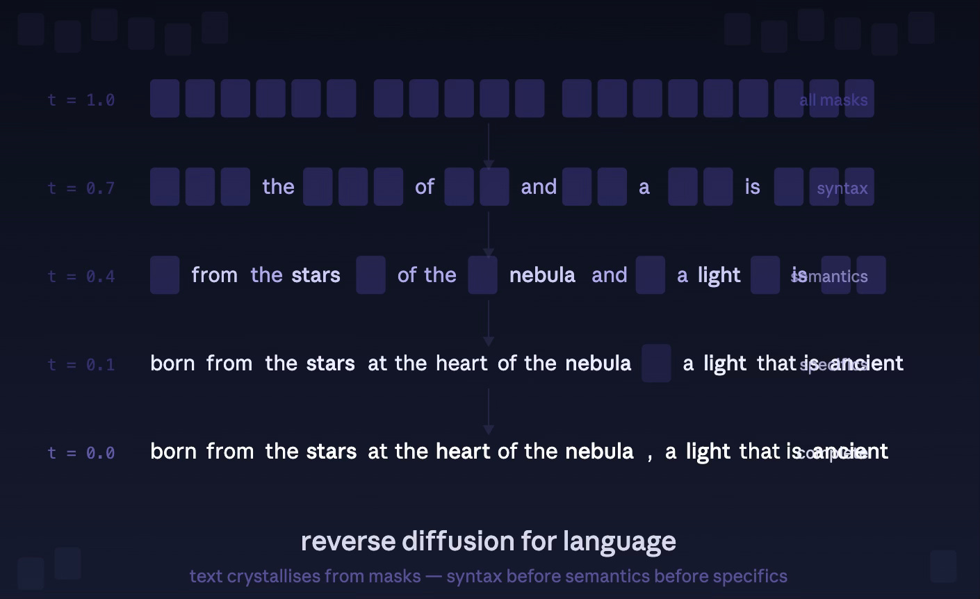
Generation is reverse diffusion. Start with all [MASK] tokens. At each step, the model predicts every position; a stochastic sampler decides which positions to unmask based on the noise schedule. Repeat until nothing is masked.
Text crystallises the same way images denoise: structure first (function words, syntax), then content (nouns, verbs, topics), then specifics (names, numbers, rare words).
Results
MDLM achieved the best perplexity among diffusion language models on both OpenWebText and LM1B. On OpenWebText with 1M training steps, it reached a test perplexity of 30.5 which is within 14% of the GPT-2 autoregressive baseline at 29.0. On zero-shot transfer benchmarks (LAMBADA, Scientific Papers), MDLM sometimes beat the AR model, suggesting that bidirectional context provides genuine advantages for certain distributions.
Why Diffusion for Language?
If autoregressive models are already very good at language, why pursue diffusion?
Parallel generation. AR models generate one token at a time, sequentially. A 1024-token response requires 1024 serial forward passes. Diffusion models predict all positions simultaneously at each denoising step, and each step reveals multiple tokens. Google’s Gemini Diffusion (May 2025) demonstrated this at production scale: ~1500 tokens per second, approximately 5× faster than autoregressive generation.
Infilling. Given a sentence with a gap in the middle, a diffusion model can fill it in naturally, it conditions on both left and right context. This is the native inference mode. An AR model can only condition on left context; filling in a gap requires expensive tricks like iterative refinement or bidirectional beam search.
Iterative refinement. A diffusion model can generate a draft, selectively re-mask the parts it’s least confident about, and regenerate them. This is the text analog of inpainting in images. ReMDM (Wang et al., 2025) formalised this as a remasking framework and showed it improves quality with inference-time compute scaling.
The gap is narrowing. D3PM (2021) was 2–3× worse than GPT-2. SEDD (2023) matched it. MDLM (2024) came within 14%. LLaDA (Nie et al., 2025) reached parity at 8B parameters. Gemini Diffusion (2025) entered production. The trajectory is clear.
Training MDLM from Scratch
We implemented the entire MDLM pipeline from scratch in PyTorch, no framework code, no external libraries beyond the tokenizer and dataset, and trained it on OpenWebText using a single GPU.
The Implementation
Every component in plain code:
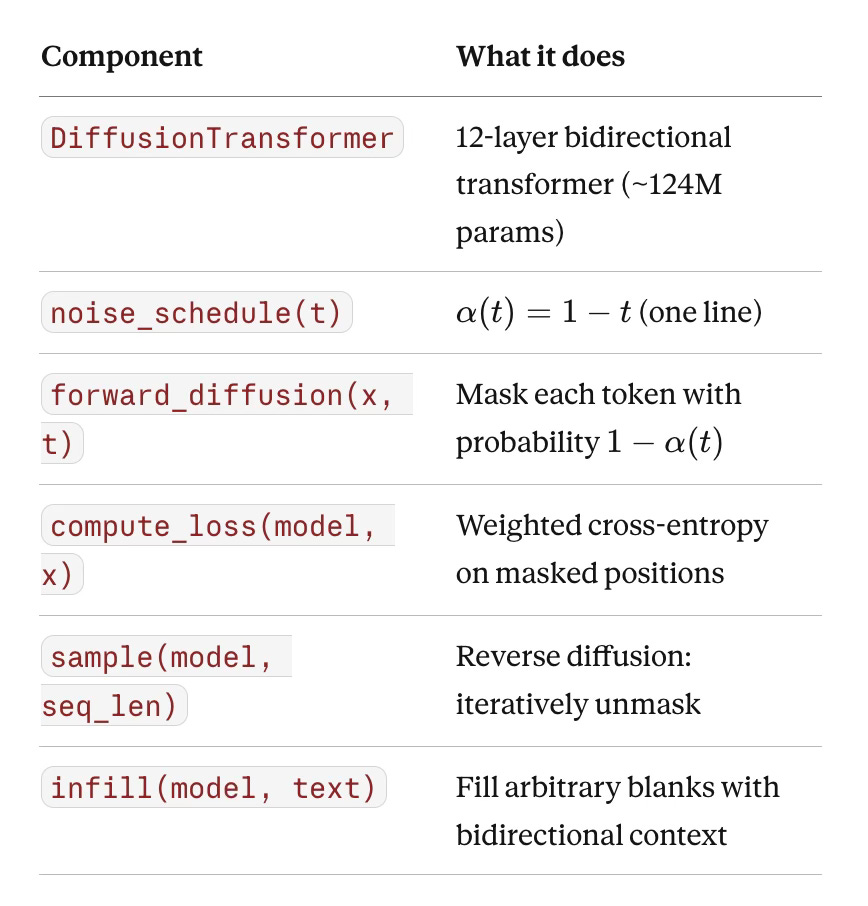
The training loop is 25 lines and mirrors the DDPM loop from Part I exactly: sample noise level, corrupt, predict, compute loss, backpropagate. The only difference: “corrupt” means “mask tokens” instead of “add Gaussian noise,” and “predict” means “cross-entropy on masked positions” instead of “MSE on predicted noise.”
Setup
We streamed OpenWebText directly from HuggingFace to avoid filling the disk —documents arrive one at a time, get tokenized with the GPT-2 tokenizer (50,257 vocabulary), and are packed into 1024-token chunks on the fly. The model trained with AdamW, learning rate 3×10^−4, cosine schedule, bfloat16 mixed precision, gradient accumulation to an effective batch size of 128.
Training Dynamics
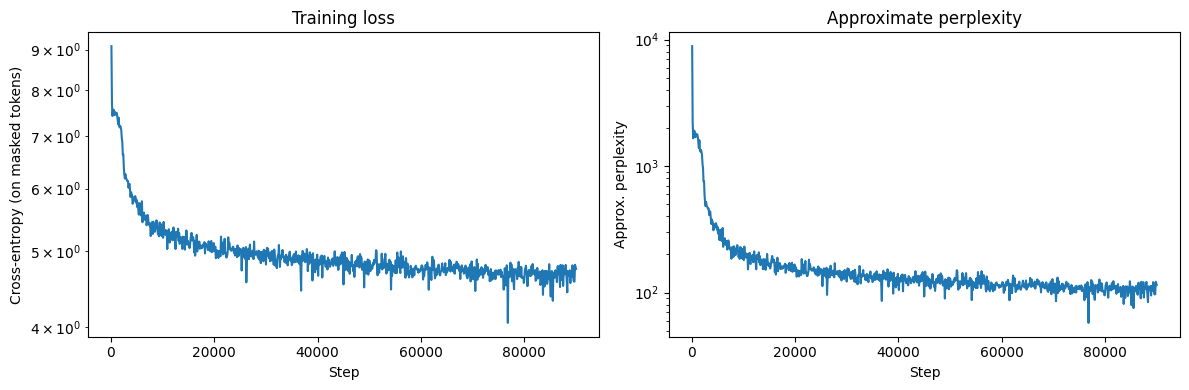
At 100,000 steps (~12B tokens processed), the model had trained for approximately 20 hours on a single A100. The training loss curve shows the expected pattern: rapid descent for the first 10K steps as the model learns basic token statistics, then a slower, steady decline as it learns grammatical structure and topical coherence.
The generated text at different checkpoints tells the story clearly:
At 50K steps, the model generates grammatical sentences that maintain a topic for one or two sentences before drifting. Repetition is the dominant failure mode — the model latches onto a word or phrase and can’t escape. Here’s a representative sample:
on the front and straight. Leave the structure for a finish or a rebuild. The left side has the same structure as the alignment of that alignment...
Grammatical. Topical (construction/building). But repetitive and shallow.
At 100K steps, a noticeable improvement. Topics are sustained across full paragraphs, vocabulary is more diverse, and the model handles different registers:
usually just send an HTML Link Buffer that helps relay the user’s feedback for ideas. As I think of the above, theAMP for which is like. It sends the questions visitors care about, whenever they’ve been submitted...
and made its first attack on September 9, 2010. It was named after two zombie attacks last year on top of Libin Hall, on September 10, 2010, and September 11...
The web-text flavour of OpenWebText is clearly present — technical jargon, conversational asides, date-specific claims. The model has absorbed the distribution. The repetition collapses that dominated at 50K are much rarer, though they still appear in some samples.
Watching Language Crystallize
The most instructive visualization is the unmasking process — the discrete analog of the denoising filmstrip from Parts I and II. We start with 128 [MASK] tokens and run reverse diffusion for 128 steps, capturing the sequence at intervals.
Here is what the model produced at 90K steps (▒ represents [MASK]):
Step 0 (0% unmasked):
▒▒▒▒▒▒▒▒▒▒▒▒▒▒▒▒▒▒▒▒▒▒▒▒▒▒▒▒▒▒▒▒▒▒▒▒▒▒▒▒▒▒▒▒▒▒▒▒▒...
Step 16 (12% unmasked):
▒▒▒▒▒▒▒▒▒▒▒▒▒▒▒▒▒▒ an▒▒▒▒▒▒ with▒▒▒ I▒▒▒▒.▒▒▒▒▒▒
▒▒▒▒▒▒▒▒▒▒▒▒▒▒ partner▒▒▒▒ the▒▒▒▒▒ You▒▒▒ ▒▒▒▒ve
▒▒▒▒▒▒▒▒ you▒▒▒▒▒▒▒▒▒▒▒▒▒▒▒▒ I▒▒▒▒ you▒ a virgin.▒▒▒▒▒
Step 48 (39% unmasked):
▒ is a▒▒▒▒ . ▒ partner. This▒ been▒▒ this▒ an▒-▒▒▒▒ with
▒ partners. I▒ it▒▒.▒▒▒▒▒▒▒ partner▒▒▒▒ve▒▒ . . ...
Step 80 (61% unmasked):
▒ is a▒▒▒▒ .▒ partner. This▒ been done because this is an▒
-▒-▒▒ with multiple partners. I▒ it for you.▒▒▒ve▒▒ a partner...
Step 127 (100% unmasked):
This is a two-part . . . partner. This has been done because
this is a two-part-times relationship with multiple partners.
I love it for you. You've also been a partner. You've . . . .
In New York, I'm a partner...
Watch the hierarchy:
Function words first (steps 0–16): “an,” “with,” “I,” “the,” “You,” “a” — pure syntactic scaffolding with no semantic content. The model’s first decisions are about sentence structure.
Topic crystallization (steps 16–48): “partner,” “virgin” — the model commits to a subject. Like image diffusion resolving the overall composition before the details, the language model determines what the text is about before what it says.
Structure and grammar (steps 48–80): “This has been done because this is an... with multiple partners” — the model fills in connective tissue, establishing grammatical relationships between the topic words.
Specifics last (steps 80–127): “two-part,” “New York,” “I love it for you” — the final details, analogous to texture in image generation.
This is the same coarse-to-fine hierarchy we observed in Parts I and II, now operating in discrete token space. Composition before content. Structure before specifics. And the model discovered this hierarchy entirely on its own, we never told it to generate function words first.
Infilling
The infilling capability works by providing a partial sequence with some positions masked and running reverse diffusion only on the masked positions. The surrounding context (both left and right) conditions the generation through bidirectional attention.
At 100K steps, the model produces:
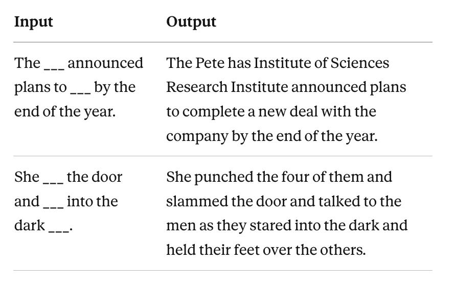
The fills are imperfect, the model is undertrained and some outputs are incoherent, but the mechanism is clearly working. The second example is genuinely compelling: “punched,” “slammed,” “stared into the dark” create a coherent narrative with consistent tone, conditioned on both the left context (”She”) and the right context (”the door,” “into the dark”). An autoregressive model would have to generate left-to-right and could not condition on “into the dark” when choosing “punched.”
With the fully trained model (1M steps), these fills become sharp and contextually appropriate.
Broader Landscape
Our experiment is a small point on a rapidly moving frontier. The field has accelerated dramatically since MDLM:
LLaDA (Nie et al., February 2025) scaled masked diffusion to 8 billion parameters and demonstrated, for the first time, that diffusion language models can match autoregressive models at sufficient scale. The architecture is MDLM’s masking framework with a larger transformer backbone. The result settles the question of whether the diffusion–AR performance gap is fundamental (it isn’t) or a scaling artifact (it is).
BD3-LM (Arriola et al., ICLR 2025 Oral) introduced block diffusion — a hybrid that applies causal attention betweenblocks and bidirectional attention within blocks. This interpolates between autoregressive (block size 1) and fully diffusive (block size = sequence length) generation, enabling arbitrary-length sequence generation while retaining the quality advantages of both paradigms.
Gemini Diffusion (Google, May 2025) brought discrete diffusion to production. Running at approximately 1,500 tokens per second — roughly 5× faster than autoregressive generation — Gemini Diffusion demonstrated that the speed advantages of parallel decoding translate to real-world gains. It matches autoregressive performance on coding benchmarks and shows strong mathematical reasoning.
The trajectory is unmistakable. D3PM (2021) proved the concept but performed poorly. SEDD (2023) closed half the gap. MDLM (2024) closed most of the rest. LLaDA (2025) reached parity. Gemini Diffusion (2025) entered production. Each step: simpler, more performant, more practical.
Arc
Let’s step back and see the full picture across all three parts.
Part I: An ink drop dissolves in water. We learn to reverse entropy with Langevin dynamics and score matching. The score function — the gradient of the log probability — is the fundamental object. We train DDPM on MNIST and watch digits emerge from noise, coarse structure first, fine detail last.
Part II: We go inside Stable Diffusion. Cross-attention maps language to spatial features. Classifier-free guidance steers the reverse process. U-Nets give way to Diffusion Transformers. We teach the model Haeckel’s aesthetic with a 1% parameter perturbation. The denoising filmstrip shows the same hierarchy at 1024×1024: composition before objects before texture.
Part III: We cross into language. The continuous machinery breaks — you can’t add Gaussian noise to a word. The field converges on masking as the discrete analog of noise, and discovers that BERT’s training objective is discrete diffusion. We build the whole thing from scratch and watch text crystallize from masks with the same coarse-to-fine hierarchy: syntax before semantics before specifics.
The same mathematical framework. The same training loop structure. The same coarse-to-fine generation hierarchy. Different media, same physics.
And the two sides are now converging. Diffusion Transformers serve both modalities. Flow matching applies to both continuous and discrete transport. The vision of a single generative framework that handles images, text, audio, molecules, and protein sequences — all through iterative refinement from noise to data — is no longer speculative. It is the direction the field is heading.
The complete training notebook (from-scratch PyTorch, streaming OpenWebText, single-GPU) is available upon request. Model weights at 100K steps are on the HuggingFace Hub. The implementation is ~150 lines of model code, ~50 lines of training loop, and zero external frameworks.
References
Austin, J., Johnson, D., Ho, J., Tarlow, D., & van den Berg, R. (2021). Structured Denoising Diffusion Models in Discrete State-Spaces (D3PM).
Lou, A., Meng, C., & Ermon, S. (2023). Discrete Diffusion Modeling by Estimating the Ratios of the Data Distribution (SEDD). ICML 2024 Best Paper.
Sahoo, S.S., Arriola, M., Schiff, Y., Gokaslan, A., Marroquin, E., Rush, A., Chiu, J.T., & Kuleshov, V. (2024). Simple and Effective Masked Diffusion Language Models (MDLM). NeurIPS 2024.
Nie, S., et al. (2025). Large Language Diffusion Models (LLaDA).
Arriola, M., Gokaslan, A., Chiu, J.T., et al. (2025). Block Diffusion: Interpolating Between Autoregressive and Diffusion Language Models (BD3-LM). ICLR 2025 Oral.
Wang, G., Schiff, Y., Sahoo, S., & Kuleshov, V. (2025). Remasking Discrete Diffusion Models with Inference-Time Scaling (ReMDM).
Li, X.L., Thickstun, J., Gulrajani, I., Liang, P., & Hashimoto, T.B. (2022). Diffusion-LM Improves Controllable Text Generation.
Devlin, J., Chang, M.W., Lee, K., & Toutanova, K. (2018). BERT: Pre-training of Deep Bidirectional Transformers for Language Understanding.
Ho, J., Jain, A., & Abbeel, P. (2020). Denoising Diffusion Probabilistic Models.
Song, Y. & Ermon, S. (2019). Generative Modeling by Estimating Gradients of the Data Distribution.
Lipman, Y., Chen, R.T.Q., Ben-Hamu, H., Nickel, M., & Le, M. (2023). Flow Matching for Generative Modeling.
If you find this post useful, I would appreciate if you cite it as:
@misc{verma202diffusion-models-iii,
  title={Diffusion Models - III: Language Models
  year={2026},
  url={\url{https://januverma.substack.com/p/diffusion-models-iii-language-models}},
  note={Incomplete Distillation}
}