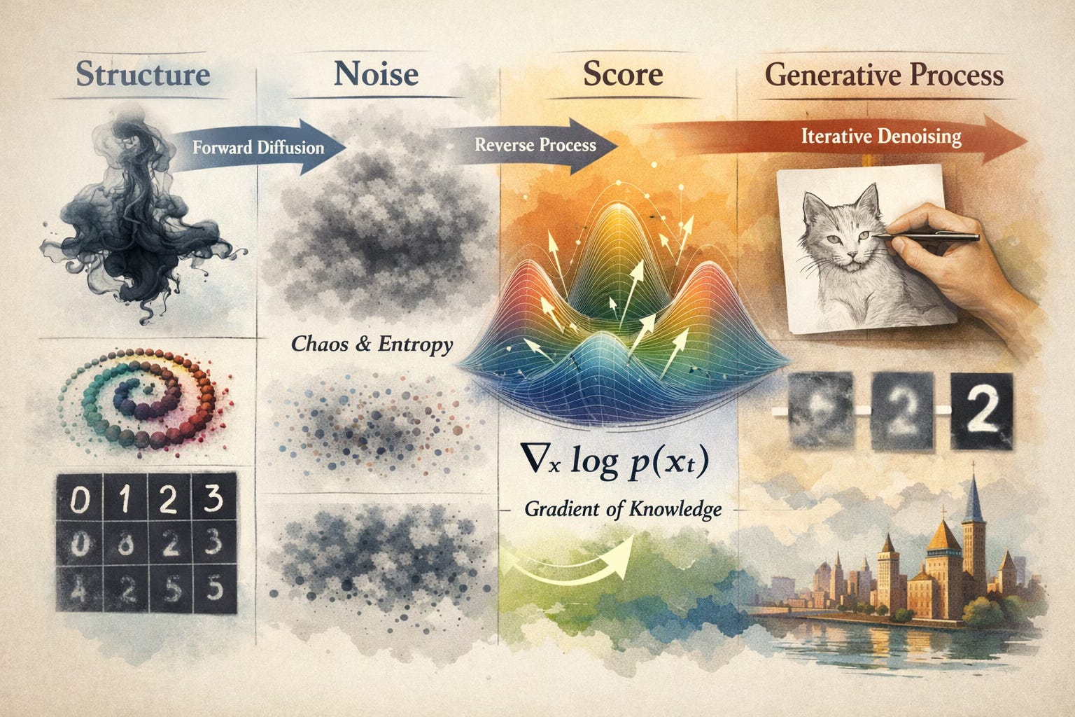
Diffusion Models: From Thermodynamics to Language

Destroying structure is easy. Reversing it is the trick.

Irreversibility in Physics

Drop a single bead of ink into a glass of still water. At the moment of contact, all the ink molecules are concentrated in one tiny region forming a highly structured, low-entropy state. Then, within seconds, the molecules bounce around randomly, colliding with water molecules, and gradually spread out into a uniform haze. We have gone from structure to noise.

Now try to reverse it. Try to coax those dispersed molecules back into a single, concentrated bead.

In principle, physics says this is possible. The fundamental laws governing molecular motion — Newton’s laws, the equations of electromagnetism, even quantum mechanics — are almost all time-reversible. If you filmed a handful of particles bouncing around and played the film backwards, both the forward and the reverse would be perfectly valid physics. There is nothing in the equations that picks out a preferred direction of time.

And yet, at the macroscopic level, we see irreversibility everywhere. Eggs break but don’t unbreak. Coffee cools but never spontaneously heats up. The ink disperses but never reconcentrates. The second law of thermodynamics (entropy tends to increase) imposes a clear arrow of time.

This tension has a name: Loschmidt’s paradox, and it was thrown at Ludwig Boltzmann in the 1870s as an objection to his statistical mechanics. How do you get irreversible macroscopic behavior from reversible microscopic laws?

The resolution is that irreversibility is statistical, not fundamental. The reverse process is not forbidden by any law of physics. But it is astronomically unlikely. When the ink is dispersed, there are an incomprehensibly vast number of molecular arrangements that all look like “uniform haze.” There is only a tiny, tiny number that look like “concentrated bead.” If the system is exploring states randomly, it will essentially never stumble back into the concentrated configuration. The reverse trajectory exists in the vast space of possibilities, but the probability of finding it by chance is something like 1 in 10^(10^23).

destruction is trivial, creation requires knowledge

This asymmetry is the deep insight behind diffusion models. The forward process (adding noise to data) is easy and requires no intelligence. You just let physics, or random number generators do their thing. The entire difficulty, and the entire art, lies in learning to run the process backwards. And to run it backwards, you need a model that has learned something about what “structure” looks like.

The Langevin Equation

Let’s make the ink drop mathematical. Consider a particle moving around randomly. At each instant, two things are happening to it: a deterministic force is pushing it somewhere, and random collisions are moving it unpredictably. The Langevin equation captures both:

\(dx = f(x)dt + g(t)dW\)

Each piece has a clear meaning:

• dx is the infinitesimal change in position. “Where does the particle move next?”

• f(x)dt is the deterministic drift. If you are on a hill, this is gravity pulling you downhill. The function f(x) encodes the direction and strength of the systematic push at position x. In the absence of noise, the particle would follow this drift smoothly and predictably.

• g(t)dW is the stochastic kick. W is a Wiener process (the mathematical formalization of Brownian motion) and dW is a tiny random increment drawn from a Gaussian with variance dt. The function g(t) controls the amplitude of the noise, and it can vary over time.

At every moment, the particle takes a step that is part deliberate (the drift) and part random (the noise). When noise dominates, the particle wanders aimlessly. When drift dominates, it follows a predictable trajectory.

The Forward Process: From Data to Noise

For the forward process that destroys structure, the diffusion models use a specific choice of Langevin equation:

\(dx = -\tfrac{1}{2}\beta(t)xdt + \sqrt{\beta(t)}dW\)

The function β(t) is called the noise schedule, and it controls the pace of the destruction. But the essential character of this equation comes from the interplay between its two terms.

The drift term, -1/2β(t)x, is a mean-reverting force. The negative sign and the proportionality to x together create a spring-like pull toward the origin:

• if x is positive, the drift is negative

• if x is negative, the drift is positive

and the further you are from zero, the stronger the pull. This is an Ornstein-Uhlenbeck process, and its effect is to exponentially shrink the signal. The expected value of x decays over time, dragging the memory of the original data toward zero.

The noise term, square root of β(t)dW, adds a fresh Gaussian kick at every instant. Each individual kick is tiny, but noise accumulates: the variances of independent random variables add, so the total noise variance grows steadily over time.

The combined effect is like trying to listen to a song while someone slowly turns down the volume and simultaneously turns up the static. The signal-to-noise ratio monotonically decreases. After sufficient time, the signal has been squashed to essentially zero, the accumulated noise dominates, and you are left with samples from approximately a standard Gaussian distribution. No trace of the original data remains.

One subtlety: β(t) appears in both terms. When β(t) is large, you are shrinking faster and adding noise faster. The noise schedule controls the overall speed of the process, not the balance between its two effects. The balance is baked into the specific coefficients (minus for drift, square root for noise), chosen precisely so that the process converges to a standard Gaussian, not one that blows up to infinite variance or collapses to zero.

The Beautiful Shortcut

Since each step is linear and Gaussian, we can write down the distribution at any arbitrary time t in closed form, without simulating the whole chain. Given a clean data point x_0, the noisy version at time t is:

\(x_t = \alpha_t x_0 + \sigma_t \varepsilon, \quad \varepsilon \sim \mathcal{N}(0, I)\)

where α_t​ is a factor that decays from 1 toward 0 (the signal shrinking) and σ_t grows from 0 toward 1 (the noise accumulating), both determined by the noise schedule β(t). This means you can jump directly from a clean data point to any noise level in a single step — a property that makes training enormously efficient.

The Score Function

We have defined a process that reliably transforms any data distribution into a standard Gaussian. Now the question that matters: can we reverse it? Can we start from Gaussian noise and recover the data?

In 1982, Brian Anderson proved something remarkable. The reverse-time stochastic process (that runs the diffusion backwards) is itself a Langevin equation:

\(dx = \left[f(x) - g(t)^2\nabla_x \log p_t(x)\right] dt + g(t)d\bar{W}\)

This is the reverse-time diffusion theorem. Look at this carefully. It is almost identical to the forward equation. The drift f(x) is there. The noise coefficient g(t) is there. But a new term has appeared:

\(g(t)^2\nabla_x \log p_t(x)\)

This term is the score function, and it is the single most important object in the theory of diffusion models.

What the Score Function Means

The score function is the gradient of the log probability density with respect to x. At every point in space, it gives you a vector which has a direction and a magnitude.

What does this vector point toward? Regions of higher probability density. If you are standing in a low-density region, far from the data, the score vector says “go this way to find more structure.” If you are standing right on top of a mode (a peak of the distribution) the score is zero, because you are already at a local maximum; there is no “uphill” direction.

Think of a topographic map where elevation represents probability density. The score function is the slope of the terrain at every point. It always points uphill.

In the reverse-time equation, the score plays the role of a restoring force. The forward drift was pushing everything toward zero, destroying structure. The score term fights against this, pointing the particle back toward the regions where data actually lives. It is the force that knows where structure is and can guide you back to it.

If you know the score at every noise level, from t = 1 (pure noise) to t = 0 (clean data), you can run Anderson’s reverse equation and transform Gaussian noise into data samples. The score is the only unknown — everything else in the equation (f, g, dWˉ) was chosen by us.

The entire field of diffusion models reduces to one problem: learn to estimate

\(\nabla_x \log p_t(x)\)

The Problem with the Score

There is a catch. We need the score of p_t(x) — the marginal distribution of noisy data at time t. This is the distribution you get by taking all possible clean data points, noising each one to level t, and mixing the results together:

\(p_t(x_t) = \int p_t(x_t \mid x_0) p_0(x_0) dx_0\)

Each p_t(x_t | x_0) term is a Gaussian (we established that the noisy version of any specific data point is Gaussian). So p_t(x_t) is a mixture of Gaussians, one for every data point in the dataset.

If you have a million training images, this is a mixture of a million Gaussians. You can write down each component, but the score of the mixture which is the gradient of the log of a sum is not the sum of the gradients of the logs. The log-of-a-sum doesn’t decompose nicely:

\(\nabla_x \log p_t(x_t) = \frac{\sum_i \nabla_x \mathcal{N}(x_t; \alpha_t x_0^i, \sigma_t^2 I)}{\sum_i \mathcal{N}(x_t; \alpha_t x_0^i, \sigma_t^2 I)}\)

Computing this requires summing over the entire dataset for every query point x_t, which is completely impractical. And even this expression approximates p_0 with the empirical dataset; the true data distribution is unknown, making the integral formally intractable.

On the other hand, the conditional score — the score given a specific clean data point x_0 — is trivial. Since

\(p_t(x_t \mid x_0) = \mathcal{N}(x_t; \alpha_t x_0, \sigma_t^2 I)\)

and the score of a Gaussian

\(\mathcal{N}(\mu, \sigma^2) \hspace{2mm} \text{is simply} \hspace{2mm} -(x - \mu)/\sigma^2\)

we get:

\(\nabla_x \log p_t(x_t \mid x_0) = -\frac{x_t - \alpha_t x_0}{\sigma_t^2} = -\frac{\varepsilon}{\sigma_t}\)

The conditional score is just the negative of the noise that was added, scaled by σ_t. One Gaussian, one line of calculus, completely known.

So we have a sharp asymmetry:

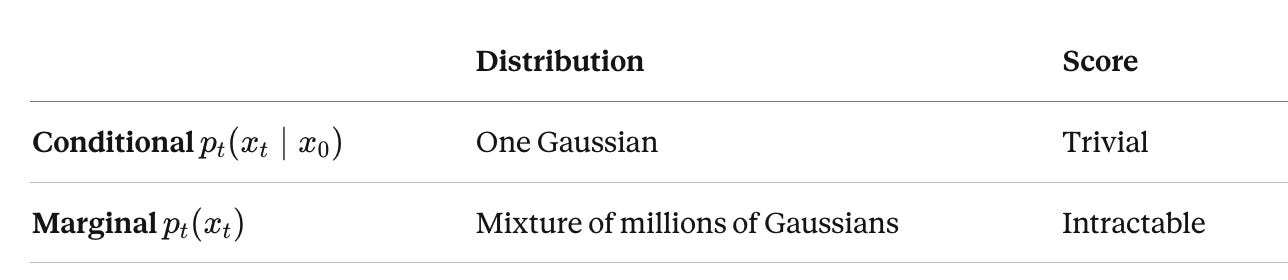
The conditional score is easy. The marginal score is the one we need. And we can’t compute it directly.

Denoising Score Matching

This is where the key insight due to Pascal Vincent (2011), building on earlier work by Aapo Hyvärinen (2005) comes in.

You can train a neural network using only the easy conditional scores, and what the network converges to after averaging over the training data provides an estimate of the hard marginal score. The procedure is almost absurdly simple:

1. Sample a clean data point x_0 from the dataset

2. Sample a random noise level t ~ Uniform(0, 1)

3. Sample noise ε ∼ N(0,I)

4. Compute the noisy version: x_t ​= α_t​ x_0​ + σ_t ​ε

5. Train a network ε_θ​(x_t​,t) to predict ε from x_t and t

6. The loss is mean squared error: |ε_θ​(x_t​,t)- ε|^2

That’s it. Add noise, predict the noise, repeat. The network that learns to predict noise is, up to a scaling factor, learning the score function at every noise level simultaneously.

Why This Works

This might feel like sleight of hand, so let me explain why predicting per-sample noise actually learns the score of the full distribution.

At any point x_t in noisy space, many different clean data points x_0 could have produced it. Each one implies a different noise vector ε (since ε = (x_t - α_t​ x_0) / σ_t). When the network trains on the denoising objective over the whole dataset, it sees x_t paired with different ε values from different source points, and it learns the expected value of ε given x_t i.e the average noise vector, weighted by how likely each clean data point was to have generated x_t.

That weighted average is:

\(\mathbb{E}[\varepsilon \mid x_t] = \sum_i w_i \cdot \varepsilon_i, \quad \text{where } w_i \propto \mathcal{N}(x_t; \alpha_t x_0^i, \sigma_t^2 I)\)

And this turns out to be exactly proportional to ∇_x​ log p_t​(x_t) — the marginal score. The network never computes the intractable sum over the dataset. Instead, stochastic gradient descent over many training steps implicitly performs this averaging, and the network converges to the right answer.

This was proven formally by Vincent, and it is what makes the entire framework work.

Seeing It — The Swiss Roll

We have the theory. Now let’s watch it work.

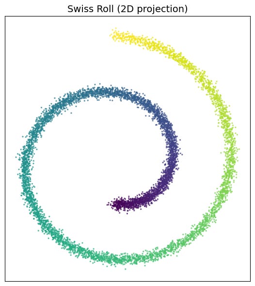
The Swiss roll is a classic dataset in machine learning: a spiral embedded in space, simple enough to visualize completely, yet with enough geometric structure to be a meaningful test. Our data consists of 8,000 points tracing out a 2D spiral, a manifold with clear, intricate structure that we can watch dissolve and, if everything works, watch re-emerge.

Why 2D? Because we can see everything. We can plot every data point, visualize the score as a vector field, and watch the reverse process unfold in real time. In higher dimensions (images, audio, text) the same mechanics are at work, but they are hidden behind thousands of dimensions. Here, nothing is hidden.

The Forward Process: Watching Structure Dissolve

Recall the forward process. Given a clean data point x_0, we can jump to any noise level t in a single step:

\(x_t = \sqrt{\bar{\alpha}_t} x_0 + \sqrt{1 - \bar{\alpha}_t} \varepsilon, \quad \varepsilon \sim \mathcal{N}(0, I)\)

The first coefficient shrinks the signal. The second grows the noise. Let’s apply this to every point in the Swiss roll at increasing noise levels and see what happens.

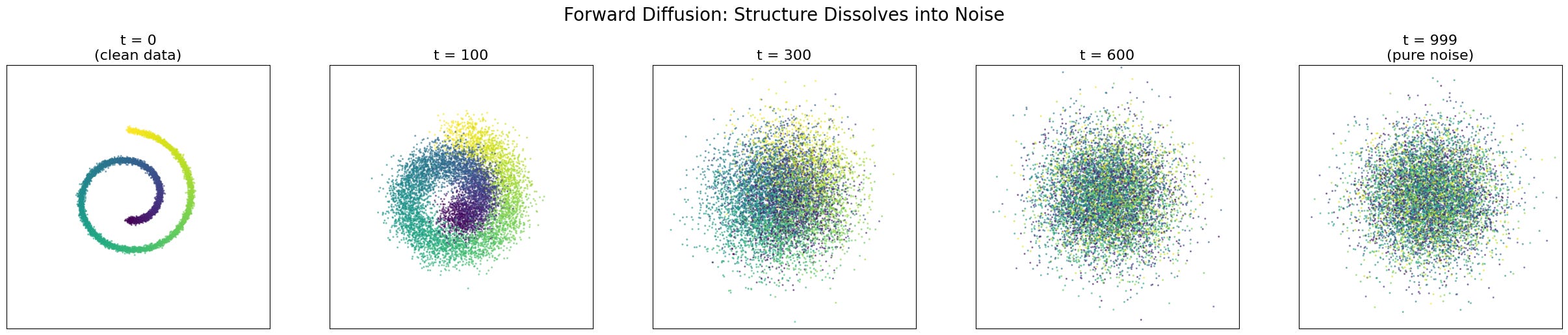
The progression is striking. At t = 0, the spiral is crisp and clearly defined. By t = 100, the edges are fuzzy but the overall shape is intact — you can still tell it is a spiral. At t = 300, the fine structure is gone; what remains is a vague, blobby memory of the original geometry. By t = 600, even that memory is fading. At t = 999, we have a shapeless Gaussian cloud. The spiral has been completely erased.

Notice that the colour (which tracks position along the original spiral) becomes progressively scrambled. Nearby points on the spiral drift apart; distant points become intermingled. The information about “where you were” in the original structure is being systematically destroyed.

This is the ink drop, made precise. And it required no learning at all — just sampling from a Gaussian.

The Score Field: A Map Back to Structure

Now for the hard part. We train a small neural network — a multi-layer perceptron with sinusoidal time embeddings — using the denoising score matching objective. The network takes a noisy point (x_t, t) and predicts the noise ε that was added. Training takes a few minutes.

What has this network learned? It has learned the score function ∇_x​ log p_t​(x_t)at every noise level which is a vector field that, at each point in space, points toward regions of higher data density. Let’s visualize it.

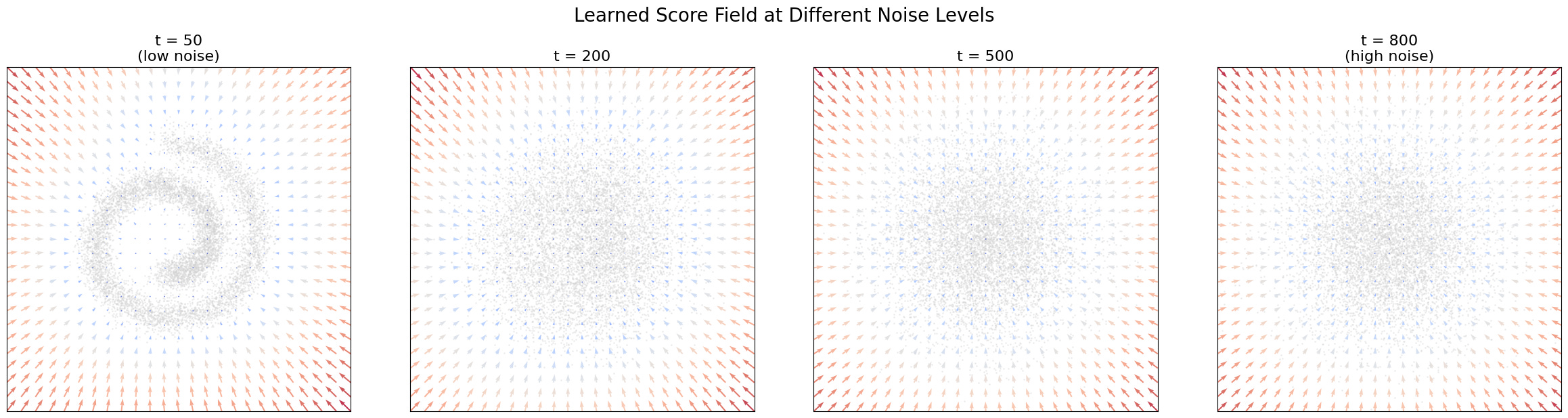
This is, to me, the most revealing visualization in the entire theory of diffusion models.

At high noise (t = 800), the data is nearly Gaussian, and the score field reflects this: the arrows point broadly inward, toward the center of mass. The network has learned little more than “the data is somewhere around the origin.” This is coarse, global information.

At medium noise (t = 500), something more interesting emerges. The arrows still point generally inward, but they are starting to curve. The network is beginning to sense the large-scale shape, that the data isn’t just a blob, but has some elongated, curved structure.

At lower noise (t = 200), the spiral geometry becomes visible in the score field. The arrows trace the curvature of the spiral arms, guiding points not just toward the center but along the manifold. The network knows the shape.

At low noise (t = 30), the field is sharp and detailed. The arrows point precisely toward the nearest arm of the spiral. If you are between two arms, the score field tells you which one you are closer to. The fine structure of the data is fully encoded.

This is hierarchical knowledge, learned automatically from the denoising objective. Nobody told the network to first learn coarse structure and then fine structure. It emerged naturally from the fact that at high noise levels, fine details are invisible, the only signal that survives the noise is the large-scale geometry. At low noise levels, the data is nearly clean, and the network can resolve fine details. The noise level acts as an automatic curriculum, from coarse to fine.

The Reverse Process: Noise Becomes Spiral

We have the score. Now we can run Anderson’s reverse-time equation. Starting from 5,000 points of pure Gaussian noise, we iterate the denoising step. At each step, the network predicts the noise component, we subtract it (partially), and we add a small amount of fresh noise. Step by step, from t = T back to t = 0.

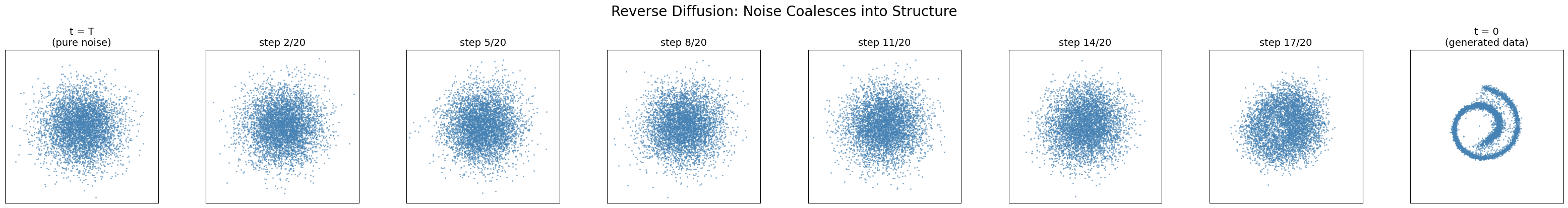
Watch what happens. The initial Gaussian cloud doesn’t snap into a spiral all at once. It organizes gradually:

Early steps (high t): The points drift inward from the Gaussian cloud, condensing into a vaguely elliptical blob. The score field is doing its coarse work, establishing that the data lives in a bounded region, roughly centered at the origin.

Middle steps: The blob starts to elongate and curve. You can begin to see the ghost of a spiral, though it’s still blurry and indistinct. The score field is now guiding points along the large-scale geometry of the manifold.

Late steps (low t): The arms of the spiral sharpen and separate. Points that were ambiguously positioned between two arms get pushed to one or the other. The fine details like the spacing between arms, the tightness of the spiral etc. snap into place.

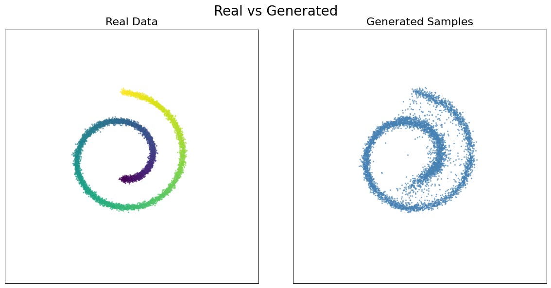
The generated samples are not copies of training data, they are new points sampled from the learned distribution. The network has captured the distribution of the Swiss roll, not memorized its individual points.

Training required nothing more than adding noise to data and training a network to predict that noise. The score function emerged as a byproduct. The hierarchical behavior i.e. coarse structure first, fine details last — was not designed but is a consequence of the physics. We demonstrated this on a 2D spiral because we could see everything. But the same mechanics operate identically in 50,000 dimensions (images) or a million dimensions (video). The only thing that changes is the architecture of the score network — from our small MLP to a U-Net or a transformer. The mathematics, the training procedure, and the sampling algorithm are exactly the same.

DDPM — Denoising as Generation

In the preceding sections, we built diffusion models from the perspective of stochastic differential equations and score matching. We started with physics, the Langevin equation, the score function, Anderson’s reverse-time SDE, and arrived at a training algorithm:

predict the noise, learn the score.

Now we come to the same place from a completely different direction. In 2020, Jonathan Ho, Ajay Jain, and Pieter Abbeel published a paper called Denoising Diffusion Probabilistic Models (DDPM) that arrived at essentially the same training algorithm, but from the tradition of variational inference rather than score matching. Their framing is more intuitive, their paper is what made diffusion models practical, and their core idea is disarmingly simple:

what if generation is just denoising, applied many, many times?

The DDPM Framing

Forget SDEs for a moment. Here is the DDPM picture.

Define a Markov chain that adds a small amount of Gaussian noise at each step. Start with a clean data point x_0 e.g. an image. At step 1, add a tiny amount of noise to get x_1. At step 2, add a bit more to get x_2. Continue for T steps (typically T = 1000). By the end, x_T is indistinguishable from pure Gaussian noise.

Each step is simple:

\(x_t = \sqrt{1 - \beta_t} x_{t-1} + \sqrt{\beta_t} \varepsilon_t\)

where ε ∼ N(0,I) and β(t) is a small noise coefficient that increases gently over time. This is just “shrink the signal slightly, add a little noise” — the same operation, repeated a thousand times.

Now the question:

can we learn to run this chain backwards?

If we had a model that could take x_t which is a noisy image and produce x_{t-1}, a slightly less noisy image, then we could start from pure noise x_T ∼ N(0,I) and iterate this denoiser T times to produce a clean image x_0.

This is the entire idea.

Generation is iterated denoising.

The Variational Perspective

Ho et al. derived the DDPM training objective through variational inference. Each step of the reverse chain can be viewed as a small variational autoencoder (VAE). The “encoder” is the forward process (add noise):

\(q(x_t | x_{t-1})\)

and the “decoder” is the learned reverse process (remove noise):

\(p_\theta(x_{t-1} | x_t)\)

The full model, chaining T such steps, is a hierarchical VAE with T levels of latent variables where the latent variables are the intermediate noisy images x_1, x_2, …, x_T.

The variational lower bound (ELBO) for this hierarchical model decomposes into a sum of T terms, one per step. Each term is a KL divergence between the true reverse step and the learned reverse step. Since both are Gaussian, this KL divergence reduces to an MSE between their means.

Working through the algebra, the mean of the true reverse step can be expressed in terms of the noise ε that was added. So training the model to predict ε from x_t and t minimizes the variational bound. This is exactly the same training objective we derived from score matching but arrived at through an entirely different route.

The Simplification That Made It Work

The full variational bound has a weighting that gives different importance to different timesteps. Ho et al. made a crucial empirical discovery: ignoring these weights and using the plain, unweighted MSE loss produced better samples. The simplified loss:

\(\mathcal{L}{\text{simple}} = \mathbb{E}{x_0, t, \varepsilon}\left[|\varepsilon - \varepsilon_\theta(x_t, t)|^2\right]\)

This is the loss we have been using throughout: sample a random timestep, add noise, predict the noise, minimize MSE. Ho et al. showed that this stripped-down objective, despite being a looser bound on the log-likelihood, produced sharper and more visually compelling samples. Sometimes less theory leads to better results.

Two Roads to the Same Algorithm

Here is something remarkable. The score matching community (Song & Ermon) started from the score function and Langevin dynamics. The variational inference community (Ho et al.) started from hierarchical VAEs and the ELBO. They used different mathematical frameworks, different notation, different conceptual vocabularies. And they arrived at the same training algorithm: sample noise, add it to data, train a network to predict it.

The deep reason is that predicting the noise is mathematically equivalent to estimating the score, up to a known scaling factor:

\(\nabla_x \log p_t(x_t) \approx -\frac{\varepsilon_\theta(x_t, t)}{\sqrt{1 - \bar\alpha_t}}\)

Score matching and DDPM are the same model viewed through different lenses. This convergence that two independent intellectual traditions arriving at identical practical algorithms is a strong signal that the underlying idea is natural and robust.

Hierarchical Denoising: The Coarse-to-Fine Story

The most important conceptual insight in DDPM is not a mathematical one, it is a perceptual one. When the reverse process generates an image, it does so in a natural coarse-to-fine hierarchy:

Early steps (high noise, t near T): The model is working with data that is almost pure noise. The only features that survive this level of corruption are the largest-scale, lowest-frequency structures i.e. the overall layout, the dominant colours, the rough spatial arrangement of mass. The model’s job at these steps is to make coarse, global decisions: is the background light or dark? Is there an object in the center or distributed across the frame?

Middle steps (medium noise): The coarse structure is established, and the model begins resolving mid-level features. Object shapes emerge. The distinction between a face and a landscape becomes clear. Spatial relationships between parts are determined. The model is committing to what the image is.

Late steps (low noise, t near 0): The global and mid-level structure is locked in. The model’s job is now to add fine details i.e. sharp edges, textures, precise colours, small features like eyes or text. These high-frequency details would have been invisible under high noise, so they can only be resolved once the noise level is low enough for them to matter.

This hierarchy is not designed. Nobody told the model to handle coarse features first and fine features last. It emerges from the mathematics: at noise level t, the score function can only encode features whose spatial scale is large enough to be detectable through the noise. High-frequency details are drowned first and recovered last.

This is why watching a diffusion model generate an image has that characteristic feel — the ghostly outline appearing first, then solidifying, then sharpening into crisp detail. It is the reverse of the forward process, which destroyed details first and structure last.

Seeing the Hierarchy on MNIST

All the theory above predicts a specific, testable behavior: at each noise level, the model’s “best guess” of the clean data should reveal a hierarchy from blurry and generic (high noise) to sharp and specific (low noise). Let’s verify this directly.

We train a small U-Net (scaled down to under two million parameters) on MNIST handwritten digits using the DDPM training algorithm. The key experiment: take a clean digit, corrupt it to various noise levels, and ask the model to predict the clean image. What the model predicts (the denoised estimate) reveals what information it has extracted from the noisy input.

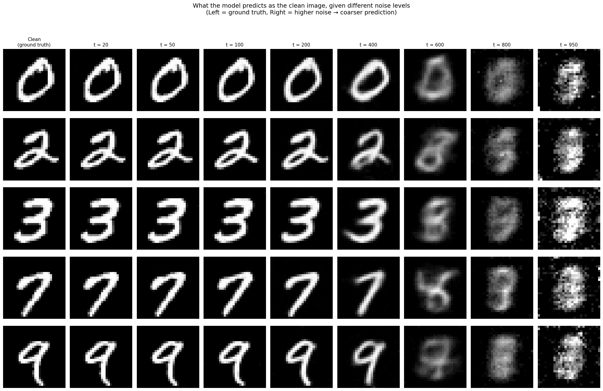
The hierarchy is unmistakable.

At t = 20, the prediction is nearly pixel-perfect, every stroke detail preserved. At t = 50 to t = 100, predictions remain sharp but subtly soften. The model is beginning to blend its observation with its prior over digit shapes. At t = 200 to t = 400, class identity is clear, you can immediately tell a 0 from a 7, but the specific instance is fading. The model’s 3 looks like a canonical, idealized 3, not this particular handwritten one. It knows what but is losing which.

At t = 600, predictions become ghostly blobs. You can still vaguely guess the class, but these are the model’s prior beliefs — what it thinks a “typical” digit looks like — weakly modulated by the faint surviving signal. At t = 800 to t = 950, the predictions are formless smudges, and something telling happens: different digits start to look alike. A heavily noised 2 and a heavily noised 7 produce similar blobs, because with that little signal, those classes are genuinely ambiguous. The model resolves these ambiguities progressively as noise decreases, first committing to a class, then to an instance, then to the fine details.

This is DDPM’s hierarchical denoising, made visible. On 28×28 digits, the effect is already striking. But the same mechanism operates at every scale and in the next section, we will see how DDPM was transformed into Stable Diffusion, where this hierarchy spans from “sky at top, ground at bottom” to “individual blades of grass.”

Latent Diffusion

DDPM established the conceptual framework: generation is iterated denoising. But DDPM itself was limited. It operated directly in pixel space, generating 32×32 or 64×64 images. Each of its 1000 denoising steps required a full forward pass through a U-Net. Scaling to high-resolution requires more efficient methods.

Running diffusion directly in pixel space is computationally brutal. A 512×512 RGB image has 786,432 dimensions. At each of the 1000 denoising steps, the U-Net must process this entire tensor. The memory and compute costs scale quadratically with image resolution (due to attention layers), making direct pixel-space diffusion impractical beyond modest resolutions.

Latent Diffusion Models (Rombach et al., 2022) solved this with a two-stage approach that separates perceptual compression from semantic generation.

Stage 1: The Autoencoder. First, train a VAE (variational autoencoder) to compress images into a much smaller latent representation. The encoder maps a 512×512×3 image to a 64×64×4 latent tensor, a 48x compression. The decoder maps it back. This autoencoder is trained separately, on a large image dataset, to reconstruct images as faithfully as possible while keeping the latent space smooth and regular.

The key insight is that most of the information in a high-resolution image is perceptually redundant. Adjacent pixels are highly correlated. The autoencoder learns to strip away this redundancy and keep only the semantically meaningful structure — edges, textures, shapes, colors — in a compact representation.

Stage 2: Diffusion in Latent Space. Now, run the entire diffusion process (forward corruption, denoising training, reverse generation) in the latent space rather than pixel space. The forward process adds noise to the latent vector. The U-Net predicts noise in latent space. The reverse process produces a clean latent vector, which is decoded to a full-resolution image the decoder.

Because the latent space is 48x smaller, every operation is dramatically faster. The U-Net never sees individual pixels, it works entirely with compressed representations. This is why Stable Diffusion can run on consumer GPUs with 8GB of VRAM, while a pixel-space model at the same resolution would require orders of magnitude more compute.

There is a subtlety worth noting: the VAE’s latent space is not learned jointly with the diffusion model. It is trained first, frozen, and then the diffusion model is trained inside this fixed space. This decoupling is what makes the approach practical, you train the expensive autoencoder once, and then many different diffusion models can operate inside the same latent space.

This is the core of text conditioned image generation methods like Stable Diffusion. The complete pipeline, from prompt to image:

1. Text encoding. The prompt e.g.“a cat sitting on a windowsill, afternoon sunlight” is tokenized and passed through (CLIP’s) text encoder, producing a sequence of 77 embedding vectors in a 768-dimensional space. These vectors encode the semantic content of the prompt.

2. Latent initialization. A random tensor z_T ∼ N(0,I) is sampled in the latent space (64×64×4). This is pure noise and forms the starting point of the reverse diffusion process.

3. Iterative denoising. For t = T, T-1, …, 1: the U-Net takes the current noisy latent z_t, the timestep t, and the text embeddings c, and predicts the noise component ε^. (Classifier-free guidance amplifies the text-conditional prediction.) The noise is partially removed according to the DDPM update rule, producing z_{t-1}. This is the reverse diffusion process, each step moves the latent slightly closer to a clean, text-consistent image.

4. Decoding. The final clean latent z_0 is passed through the VAE decoder, producing a 512×512×3 image. This single decoding step transforms the abstract latent representation into actual pixels.

This traces directly back to concepts we have developed. The iterative denoising is DDPM. The efficiency comes from operating in the VAE’s compressed latent space. And the hierarchical coarse-to-fine generation — the U-Net resolving composition before objects before textures — is the same phenomenon we saw on the Swiss roll and MNIST, now operating at production scale.

Diffusion Language Models

Everything so far has lived in continuous space. The Swiss roll is a cloud of real-valued 2D coordinates. MNIST digits are grids of pixel intensities. Gaussian noise, Langevin dynamics, the score function — all of this machinery assumes you can add a small real-valued perturbation to your data and take a gradient with respect to it.

Language is different. A sentence is a sequence of discrete tokens. You can’t add 0.01 units of Gaussian noise to the word “cat” and get something meaningful. You can’t take the gradient of a probability distribution defined over a finite vocabulary. The entire mathematical framework we’ve built seems to break down.

And yet, people have made it work.

Let’s be precise about what goes wrong. In continuous diffusion, three things happen:

1. The forward process adds Gaussian noise which requires that there is a continuous space where small perturbations make sense.

2. The score function is a gradient with respect to x which requires a continuous, differentiable space.

3. The reverse process uses the score to take small steps back toward the data. Again, continuous steps in a continuous space.

None of these work directly when x is a sequence of tokens from a finite vocabulary. There is no meaningful “halfway” between the words “cat” and “car.” The space of sentences is discrete, and the tools of calculus — which is the entire foundation of score-based diffusion — don’t apply.

There are multiple ways to handle this.

1. Absorbing State Discrete Diffusion: If you can’t add Gaussian noise, what can you do to corrupt a discrete sequence? The simplest answer: mask tokens. Replace them, one by one, with a special [MASK] token. The forward process works like this: At each timestep, every non-masked token has some probability of being replaced by [MASK]. The masking probability increases over time according to a schedule (analogous to the noise schedule). After enough steps, every token is masked. The sequence has been fully corrupted and we have the discrete analog of “pure Gaussian noise.”

   

   The reverse process is the opposite: progressive unmasking. Start with a fully masked sequence. At each step, the model examines the current state which is a mix of revealed and masked tokens, and predicts what the masked tokens should be. The most confident predictions get unmasked first. Step by step, the sequence fills in.

2. An alternative strategy is to embed discrete tokens into continuous space, run standard continuous diffusion there, and map back to tokens at the end.

   This is what Diffusion-LM (Li et al., 2022) proposed. Every token gets mapped to a continuous embedding vector (just as in any neural language model). Diffusion operates on these embeddings — adding Gaussian noise, learning the score, running the reverse SDE — and at the end, the continuous vectors are “rounded” back to the nearest discrete token.

The Deeper Connections

We have seen diffusion from two angles: score-based SDEs and DDPM-style denoising. But diffusion models touch some of the deepest ideas in mathematics and physics. These connections are underexplored in most treatments. They are also, I think, the most intellectually beautiful part of the story.

The SDE Unification

By 2020, there were two seemingly different families of diffusion models. One, descending from Sohl-Dickstein et al. (2015) and crystallized by Ho et al. (2020) in the DDPM paper, came from the variational inference tradition. The other, developed by Song and Ermon (2019), came from the score matching tradition. These two approaches used different notation, different derivations, and different sampling procedures. But they produced suspiciously similar results.

In 2021, Yang Song, Jascha Sohl-Dickstein, Diederik Kingma, Abhishek Kumar, Stefano Ermon, and Ben Poole published a paper that unified them. The key insight was deceptively simple:

both approaches are discretizations of the same underlying continuous-time process.

The forward process is a stochastic differential equation:

\(dx=f(x,t)dt + g(t)dW\)

DDPMs correspond to one particular choice of f and g (the variance-preserving SDE). Score-based models correspond to another (the variance-exploding SDE). But in both cases, Anderson’s theorem gives the reverse:

\(dx = \left[f(x,t) - g(t)^2\nabla_x \log p_t(x)\right] dt + g(t)d\bar{W}\)

Different forward SDEs lead to different noise schedules and different sampling dynamics, but the training objective is always the same: learn the score. The discrete chains of DDPM are just Euler-Maruyama discretizations of the continuous process.

This unification was clarifying, but it also revealed something unexpected.

The Probability Flow ODE. Anderson’s reverse equation is stochastic, it involves the random term g(t)dW. Song et al. showed that there exists a deterministic ordinary differential equation that has exactly the same marginal distributions p_t(x) at every time t:

\(dx=[f(x,t)−\frac{1}{2} g(t)^2 ∇_x \log⁡ p_t(x)]dt\)

No noise. No randomness. A smooth, deterministic flow that transports probability mass from the data distribution to the noise distribution (and back).

This is called the probability flow ODE, and it has remarkable consequences. Because the mapping is deterministic and invertible, it defines a continuous normalizing flow. You can compute exact log-likelihoods, something the stochastic sampler cannot do. Every data point has a unique, deterministic encoding in the noise space, giving you a latent space “for free.” And the ODE can be solved with adaptive-step solvers, opening the door to much faster sampling, instead of 1000 steps, an ODE solver might need only 20–50 function evaluations.

Optimal Transport: The Shortest Path

There is something inefficient about the diffusion process. The forward SDE takes data to noise via a random walk, a stochastic path through the space of distributions. The reverse process follows this same meandering trajectory back. But is this really the best route?

Optimal transport theory asks a cleaner question:

given a source distribution p_0 (data) and a target distribution p_1 (noise), what is the cheapest way to move probability mass from one to the other?

The answer is generally not a diffusion path. The optimal transport plan moves mass along straight lines, taking each point directly from its starting position to its destination with no detours.

This insight inspired flow matching (Lipman et al., 2023). Instead of learning to reverse a diffusion process, flow matching learns a velocity field that transports noise to data along straight (or near-straight) paths:

\(dx=v_θ(x,t)dt\)

The model v_θ is trained to regress onto the conditional velocity field that interpolates linearly between a noise sample and a data sample:

\(x_t = (1 - t)x_1 + t x_0\)

The velocity is simply v = x_0 - x_1 which is a constant pointing from noise to data in a straight line. These straight paths are far more efficient than the curved, stochastic paths of classical diffusion. The practical consequence is dramatic: flow matching models can generate high-quality samples in far fewer steps, often 20–50 instead of 1000.

This is not abstract theory. It is the reason the systems you actually use got faster. The original Stable Diffusion (v1, v2) used the classical DDPM framework and needed many denoising steps for quality results. Stable Diffusion 3 and Flux (the current state of the art) switched to flow matching. They replaced the U-Net with a Transformer (the Diffusion Transformer or DiT architecture) and replaced the DDPM SDE with rectified flow paths. This results in comparable or better image quality with dramatically fewer sampling steps, making real-time generation feasible.

The conceptual shift is subtle but important. Classical diffusion models define a physical process (noise corruption and its reversal) and learn to control it. Flow matching defines a transport problem (move this distribution to that one) and learns the optimal velocity field. Both end up training a neural network to transform noise into data, but the paths they take through the space of distributions are fundamentally different. One meanders, the other goes straight. The history of text-to-image generation, from DDPM through Stable Diffusion to Flux, is in part the history of this shift from physics to transport.

The Schrödinger Bridge: The Question Behind Everything

In 1931, Erwin Schrödinger posed a beautiful problem.

Imagine you observe a cloud of particles distributed as p_0 at time t = 0, and then you observe the same particles distributed as p_1 at time t = 1. You don’t see what happens in between. The particles undergo Brownian motion (random diffusion). Schrödinger asked: what is the most likely stochastic evolution that connects p_0 to p_1?

This is exactly the problem of generative modeling with diffusion. We have a data distribution p_0 and a noise distribution p_1 = N(0,I), and we want to find a stochastic process that connects them.

Standard diffusion models solve a simplified version of this problem. They fix the forward process and only learn the reverse. This is convenient, the forward process is known analytically, so training is easy. But it is not optimal. The forward process was chosen for mathematical convenience, not because it is the best way to bridge the two distributions.

The Schrödinger bridge formulation asks for the optimal pair i.e. the best forward and the best backward process jointly. The solution minimizes the KL divergence from the Brownian reference process, which can be interpreted as finding the most likely stochastic evolution, or equivalently, the minimum-entropy path between the two distributions.

This connects to entropic optimal transport. Classical optimal transport finds the cheapest deterministic map. Entropic optimal transport adds a regularization term that encourages some stochasticity. In the limit of zero regularization, you get optimal transport (straight lines). In the limit of infinite regularization, you get Brownian motion (pure diffusion). The Schrödinger bridge lives in between, the sweet spot that balances efficiency and randomness.

The Schrödinger bridge perspective reframes the entire enterprise. It provides a unifying view where classical diffusion, flow matching, and optimal transport are all special cases:

• Pure diffusion (DDPM, score-based models): fix the forward process, learn only the reverse. High entropy, potentially inefficient paths.

• Optimal transport / flow matching: deterministic paths, zero entropy. Maximally efficient but no stochasticity.

• Schrödinger bridge: the full solution, interpolating between these extremes.

The field is, in a sense, converging on the Schrödinger bridge as the most general framework, with the other approaches as special cases chosen for computational convenience.

Closing: The Arc

We began with a bead of ink dissolving in water and the thermodynamic observation that destruction is easy while creation requires knowledge. We formalized this as a Langevin equation, discovered that the score function is the one object needed to reverse the process, and learned that a neural network can estimate the score by simply predicting noise.

We saw this in action on a 2D spiral, where the score field visibly guides noise back into structure. We saw it on handwritten digits, where the hierarchical nature of denoising became vivid — global shape before class identity before fine detail. We traced how DDPM arrived at the same algorithm from variational inference, how latent diffusion and classifier-free guidance turned it into Stable Diffusion, and how flow matching and the Schrödinger bridge revealed the deeper mathematical landscape beneath.

The field is moving fast. Flow matching is challenging classical diffusion for efficiency. The Schrödinger bridge is being rediscovered as the unifying framework behind it all. And a question we haven’t addressed hangs in the air: what happens when you try to diffuse something discrete — language, protein sequences, molecular structures? Can you add noise to a word? In a follow-up post, I’ll confront that frontier.

For now, the core idea is simple, and it echoes through everything we have built: if you know the way back to structure, you can start from noise and create anything.

References

• Sohl-Dickstein, J., Weiss, E., Maheswaranathan, N., & Ganguli, S. (2015). Deep Unsupervised Learning using Nonequilibrium Thermodynamics.

• Hyvärinen, A. (2005). Estimation of Non-Normalized Statistical Models by Score Matching.

• Vincent, P. (2011). A Connection Between Score Matching and Denoising Autoencoders.

• Song, Y., & Ermon, S. (2019). Generative Modeling by Estimating Gradients of the Data Distribution.

• Ho, J., Jain, A., & Abbeel, P. (2020). Denoising Diffusion Probabilistic Models.

• Hu, E.J., Shen, Y., Wallis, P., Allen-Zhu, Z., Li, Y., Wang, S., Wang, L., & Chen, W. (2021). LoRA: Low-Rank Adaptation of Large Language Models.

• Song, Y., Sohl-Dickstein, J., Kingma, D.P., Kumar, A., Ermon, S., & Poole, B. (2021). Score-Based Generative Modeling through Stochastic Differential Equations.

• De Bortoli, V., Thornton, J., Heng, J., & Doucet, A. (2021). Diffusion Schrödinger Bridge with Applications to Score-Based Generative Modeling.

• Ho, J. & Salimans, T. (2022). Classifier-Free Diffusion Guidance.

• Radford, A., Kim, J.W., Hallacy, C., et al. (2021). Learning Transferable Visual Models From Natural Language Supervision (CLIP).

• Rombach, R., Blattmann, A., Lorenz, D., Esser, P., & Ommer, B. (2022). High-Resolution Image Synthesis with Latent Diffusion Models.

• Podell, D., English, Z., Lacey, K., et al. (2023). SDXL: Improving Latent Diffusion Models for High-Resolution Image Synthesis.

• Esser, P., Kulal, S., Blattmann, A., et al. (2024). Scaling Rectified Flow Transformers for High-Resolution Image Synthesis (Stable Diffusion 3).

• Lipman, Y., Chen, R.T.Q., Ben-Hamu, H., Nickel, M., & Le, M. (2023). Flow Matching for Generative Modeling.

• Liu, X., Gong, C., & Liu, Q. (2023). Flow Straight and Fast: Learning to Generate and Transfer Data with Rectified Flow.

---

If you find this post useful, I would appreciate if you cite it as:

@misc{verma202diffusion-models,   
  title={Diffusion Models: From Thermodynamics to Language
  year={2026},   
  url={\url{https://januverma.substack.com/p/diffusion-odels-from-thermodynamics}},   
  note={Incomplete Distillation} 
}