Semantic IDs for Recommendation Systems: A Technical Deep Dive

Introduction

Recommendation systems are the backbone of personalized digital experiences, guiding users through vast catalogs on platforms like Netflix, Amazon, and Spotify. At their core, these systems rely on modeling user-item interactions, historically represented in a matrix where rows correspond to users and columns to items. Each entry in this matrix captures an interaction - a clicsk, purchase, rating, or view - linking a user to an item via their respective identifiers (IDs). For instance, User 5489 might rate Item 98124, a sci-fi movie, with five stars. These IDs, however, are arbitrary, content-agnostic labels - mere placeholders that distinguish one entity from another without encoding any intrinsic meaning. Yet, these simple IDs have been the fundamental building blocks for some of the most powerful recommendation algorithms ever created.

The advent of embedding-based methods revolutionized recommendation systems. Instead of treating IDs as simple keys, models learn dense vector representations, or embeddings, for each user and item. These embeddings are stored in lookup tables, where each ID maps to a vector of fixed dimension (e.g., 32 or 64). The model learns these embeddings by trying to predict user-item interactions. For a given user ID and item ID, the system fetches their respective embedding vectors. The dot product of these two vectors is then used to predict how likely the user is to interact with the item. Through training on millions of historical interactions, the model adjusts the numbers in these embedding vectors, gradually encoding latent preferences for users and latent attributes for items. The ID 5489 might learn an embedding that shows a high preference for sci-fi, while item 98124might learn an embedding that marks it as a classic sci-fi movie. The system doesn't know what "sci-fi" is, but it learns a dimension in its vector space that corresponds to it.

This embedding-based paradigm has powered many successful systems but relies on a fundamental limitation: the IDs themselves are meaningless. They are arbitrary hashes that do not capture the semantic content of users or items, leading to challenges like the cold-start problem, bias toward popular items, and poor generalization across datasets. This post explores Semantic IDs, a transformative approach that replaces arbitrary IDs with discrete, content-aware representations. Leveraging techniques like Residual Quantization, Semantic IDs encode meaningful attributes, enabling more robust, scalable, and generalizable recommendation systems.

The Trouble with Traditional IDs

Using unique IDs for users and items a straightforward way to build the massive interaction matrices that are the bedrock of collaborative filtering and other classic recommendation algorithms. But as our digital world has grown more complex, the cracks in this foundation have started to show. Here are some of the key challenges of ID-based recommendation systems:

• The Cold-Start Problem: This is the classic recommender system dilemma. When a new user signs up or a new item is added to the catalog, it has no interaction history. Without this history, the model has no way of knowing what to recommend to the user or who might be interested in the new item. This results in poor initial recommendations, degrading user experience and delaying

  content discovery.

• The Long-Tail Problem: Recommendation systems are notoriously biased towards popular items. The "head" of the distribution - the blockbuster movies, the chart-topping songs - gets all the attention, while the vast "long tail" of niche content languishes in obscurity. This is because the model simply doesn't have enough data on these less popular items to learn meaningful representations.

• Scalability and Sparsity: As the number of users and items grows, the interaction matrix becomes astronomically large and incredibly sparse. This makes it computationally expensive to train and serve models, and the sparsity of the data can make it difficult to learn high-quality embeddings.

• Lack of Generalization: ID-based embeddings are inherently tied to a specific set of users and items. They don't capture any of the underlying semantic meaning of the content. This means that a model trained on one dataset can't be easily transferred to another, and it can't make recommendations based on the actual content of the items.

These limitations stem from the content-agnostic nature of traditional IDs, prompting the need for a paradigm that incorporates semantic meaning directly into the identifier.

Semantic ID

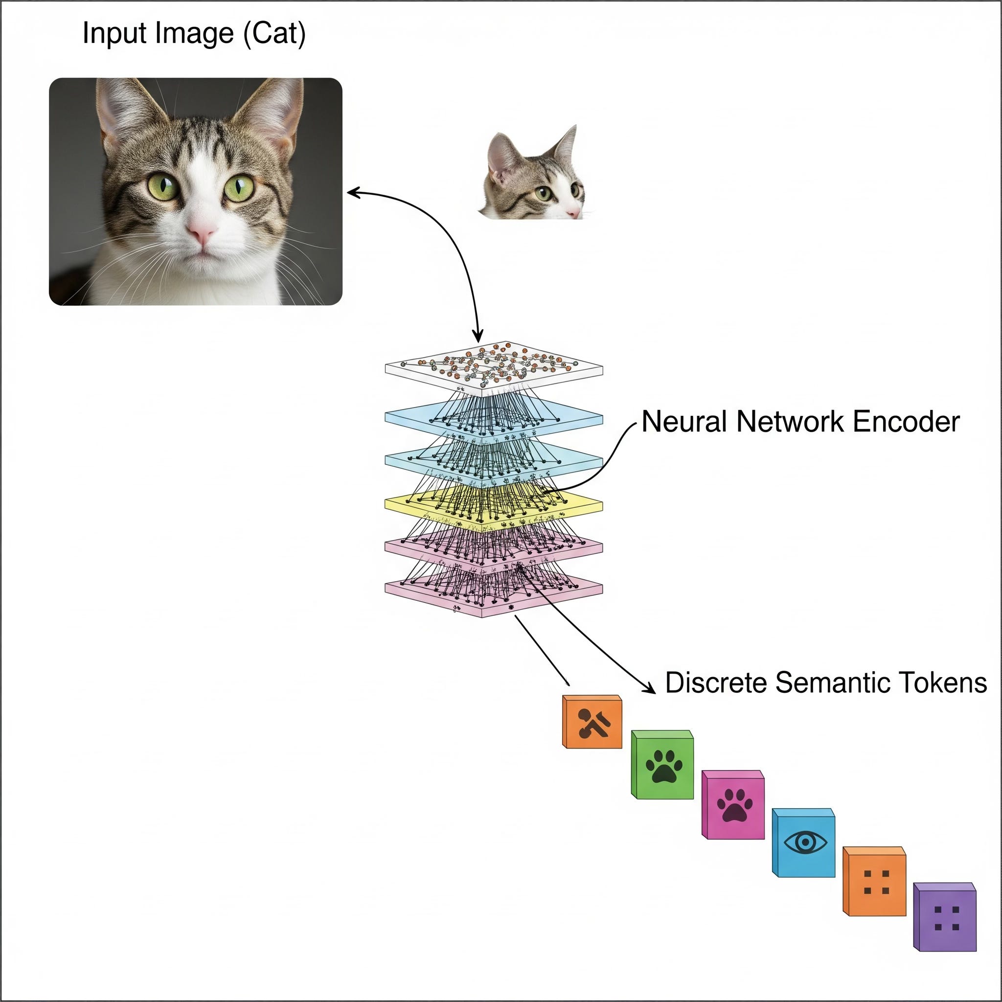
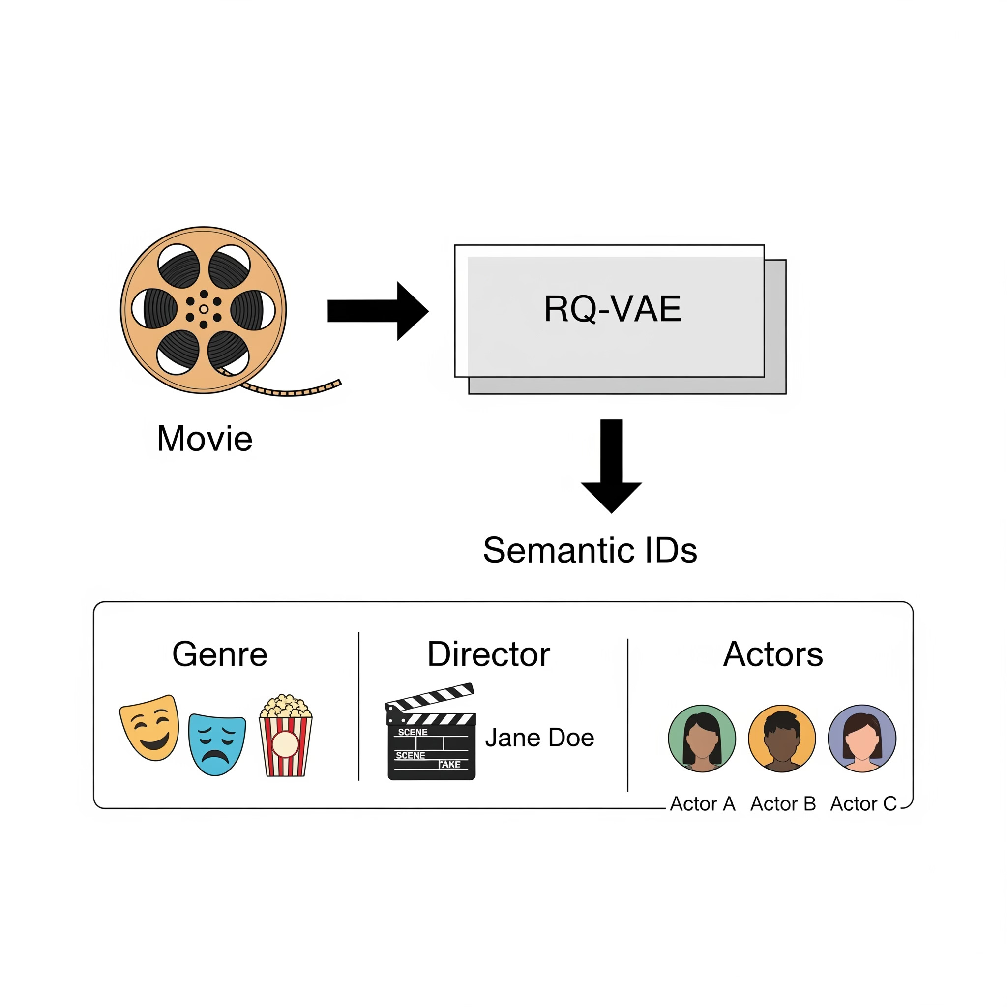
A Semantic ID is a compact, discrete representation that encodes the intrinsic content or features of an item (or user). Unlike arbitrary IDs, Semantic IDs capture meaningful attributes, enabling the system to understand similarities and differences between entities without relying solely on interaction data.

Consider two movies, Inception and Interstellar, both directed by Christopher Nolan. In a traditional system, they might be assigned IDs like 75231 and 89123, respectively, revealing nothing about their content. In contrast, a Semantic ID is a sequence of integers, each drawn from a learned codebook. For example:

• Inception: [12, 153, 87, 21]

• Interstellar: [12, 153, 87, 99]

Each integer in the sequence corresponds to a codeword from a codebook, potentially representing:

• The first code, 12, might be the codeword for the "Sci-Fi" genre.

• The second, 153, might capture a more specific sub-genre like "Heist/Thriller."

• The third, 87, could be associated with the directorial style of "Christopher Nolan."

• The final code, 21, might represent a fine-grained theme like "Dreams & consciousness."

Notice how the first three codes are identical, instantly telling the model that these two movies are very similar: they are both Nolan-directed sci-fi thrillers. The last code is different - 99 might represent the theme of "Space Travel & Relativity" - capturing the crucial difference between the two films. This is the power of a Semantic ID: it encodes both similarity and nuance directly into the item's identifier.

By using Semantic IDs, we can overcome many of the limitations of traditional ID-based systems:

• Solving the Cold-Start Problem: Because Semantic IDs are derived from the content of the items, we can generate a meaningful representation for a new item without any interaction data. This allows us to make relevant recommendations for new content right from the start.

• Unlocking the Long Tail: Semantic IDs allow us to see the similarities between items, even if they have very little interaction data. This helps us to make recommendations for niche content and to surface hidden gems from the long tail.

• Improved Generalization: Because Semantic IDs are based on the content of the items, they are much more generalizable than traditional ID-based embeddings. A model trained on Semantic IDs can be more easily transferred to new domains and new datasets.

Vector Quantization

Semantic IDs are enabled by Vector Quantization (VQ), which maps continuous embeddings to discrete codewords from a finite codebook. VQ is a classical quantization technique used in signal processing and data compression. It generalizes scalar quantization to higher dimensions by quantizing vectors instead of individual scalars. Essentially, VQ maps a multi-dimensional vector from a large vector space to a single vector from a much smaller, finite set of representative vectors. This finite set is called the codebook.

The process of vector quantization involves two main stages: encoding and decoding.

Encoding

1. Vectorization: The input data (e.g., an image or audio signal) is first partitioned into a sequence of k-dimensional vectors, x. For an image, this might involve creating vectors from non-overlapping n×n pixel blocks.

2. Nearest-Neighbor Search: For each input vector x, the encoder searches through a pre-defined codebook, C={c_1​,c_2​,…,c_N​}, to find the codeword c_i​ that is "closest" to x. The closeness is typically measured using a distortion metric, most commonly the squared Euclidean distance.

3. Quantization: The encoder then outputs the index i of this best-matching codeword. This index, which requires far fewer bits to represent than the original vector x, is what is stored or transmitted.

Decoding

The decoding process is a simple table lookup operation. The decoder receives the index i and uses it to retrieve the corresponding codeword c_i​ from its identical copy of the codebook. This codeword, x^=c_i​, serves as the reconstructed approximation of the original vector x.

The primary trade-off in VQ is between the compression rate and signal fidelity. The compression rate is determined by the size of the codebook (N) and the vector dimension (k). The fidelity is limited by the quantization error or distortion, which is the difference between the original vector x and its reconstructed approximation x^.

Learning

The most common algorithm for generating an optimal codebook is the Linde-Buzo-Gray (LBG) algorithm, which is an iterative clustering algorithm conceptually identical to k-means clustering:

1. Initialization: Select an initial set of N codewords. This can be done by randomly selecting N vectors from the training data.

2. Partitioning (Nearest Neighbor Condition): Partition the training data set into N clusters by assigning each training vector to the cluster associated with its nearest codeword (using the defined distortion metric).

3. Centroid Update (Centroid Condition): Update the codeword for each cluster by calculating the centroid (mean vector) of all training vectors assigned to that cluster. The centroid is the vector that minimizes the average distortion within the cluster.

4. Iteration: Repeat steps 2 and 3 until the average distortion converges below a certain threshold or a fixed number of iterations is reached.

While simple, this approach has a significant drawback. To achieve a fine-grained representation of the complex embedding space, you need a very large codebook (a large N). If you want to represent a billion unique items, you might need a codebook with a billion entries. This is computationally infeasible to store and search through during training and inference.

This is the problem that Residual Quantization elegantly solves.

Residual Quantization

Residual Quantization (RQ), also known as multi-stage vector quantization, builds directly on the concept of vector quantization to achieve much higher precision without an exponential increase in memory or computational cost. Instead of trying to find the single best codeword for a vector in one go, RQ refines the approximation in successive stages by quantizing the error from the previous stage.

Imagine you have a target vector x and you've already performed a standard VQ step. Your approximation isn't perfect, leaving a difference between the original vector and its quantized version. This difference is the residual error. RQ's key insight is to quantize this error as well.

Here's the step-by-step process for a two-stage RQ:

1. First Stage (Standard VQ): Quantize the original input vector x using a first-stage codebook, C_1​. This gives you the initial approximation, which is the closest codeword from C_1​.

   \(\hat{x}_1​=Q_1(x) \)

2. Calculate the Residual: Find the error vector by subtracting the approximation from the original vector.

   \(r_1​=x−x^1​ \)

3. Second Stage (Quantize the Residual): Now, treat this residual vector as a new vector to be quantized. Use a second, independent codebook, C2​, to find the best codeword that approximates this error.

   \(\hat{r}_1=Q_2(r_1​)\)

4. Final Reconstruction: The final, more accurate reconstructed vector is the sum of the codewords from both stages.

   x^=x^1​+r^1​

   \(\hat{x}=\hat{x}_1​+\hat{r}_1​\)

The original vector x is now represented by two indices: the index of the codeword from C1​ and the index of the codeword from C2​. This process can be repeated for M stages, each stage further refining the approximation by quantizing the residual of the previous stage.

The residual part is like describing a complex object in layers. Imagine describing a blue sports car.

• Level 1 Codebook (The "Object Shape" Table): This codebook has learned basic shapes. It looks at the input and picks the best match.

  • It finds that code_7 in its table, which has learned to represent a generic "car-like shape," is the best fit.

  • Semantic ID so far: [7]

• The Residual: The model now subtracts the "car-like shape" from the original input. What's left to describe? The color, the fact it's a sports car, the wheels, etc.

• Level 2 Codebook (The "Color/Style" Table): This codebook has learned properties like colors and styles. It looks at the residual error and finds the best match.

  • It finds that code_128, which represents "vibrant blue," and code_201, which represents "aerodynamic," are good fits. Let's say it picks code_128.

  • Semantic ID so far: [7, 128]

• Level 3 and 4: This continues, with each level's codebook adding another layer of detail (e.g., "has-spoiler," "shiny-texture") by describing the remaining, ever-smaller residual.

The final semantic ID [7, 128, ...] is the full recipe. The decoder then reads this recipe—"car-shape" + "vibrant blue" + ...—to reconstruct a detailed picture of the blue sports car.

The power of RQ lies in its combinatorial expressiveness. Let's say each codebook (C_1​, C_2​, ..., C_M​) contains N codewords.

• A standard VQ system with one codebook can only represent N distinct approximation vectors. To achieve higher precision, you must dramatically increase N, making the codebook huge and the search process slow.

• A Residual VQ system with M stages can represent N*M distinct approximation vectors by combining codewords from each stage.

Suppose you have two codebooks, each with 256 codewords.

• Standard VQ: You can only represent 256 vectors.

• Residual VQ (2 stages): You can represent 256×256=65,536 unique vectors by summing one codeword from the first book and one from the second.

RQ achieves a massive increase in representational power with only a linear increase in storage (storing M small codebooks instead of one giant one) and computation (performing M small searches instead of one massive search). This makes it highly effective for applications like large-scale similarity search and compressing neural network weights, where fine-grained quantization is essential.

Vector-Quantized Variational Autoencoder

A Vector-Quantized Variational Autoencoder (VQ-VAE) is a type of generative model that uses vector quantization to create a discrete latent representation of data. This elegantly solves some common problems in traditional Variational Autoencoders (VAEs) and enables the generation of remarkably high-fidelity samples. It builds directly on the principles of VQ by embedding the quantization process within a neural network.

A VQ-VAE consists of three main parts: an encoder, a vector quantization layer, and a decoder.

1. Encoder: This is a standard neural network (e.g., a Convolutional Neural Network for images) that takes an input x and maps it to a continuous latent representation Z​(x).

2. Vector Quantization (VQ) Layer: This is the core innovation. It takes the continuous output from the encoder and maps it to a discrete representation. This layer maintains a learned codebook, a list of vectors {e_1​,e_2​,…,e_K​}.

   • For each vector in the encoder's output Z(x), the VQ layer finds the closest vector e_k​ from the codebook using Euclidean distance.

   • It then passes this chosen codebook vector, now called the quantized latent vector Z_q​(x)=e_k​, to the decoder.

3. Decoder: This network takes the quantized vector Z_q​(x) and attempts to reconstruct the original input.

The key difference from a standard VAE is that the latent space is not a continuous distribution but a finite set of vectors from the codebook.

Non-Differentiability Problem

There's a significant challenge in this architecture: the process of finding the nearest neighbour (arg min) in the codebook is non-differentiable. You can't calculate a gradient for this "lookup" operation, which means you can't use standard backpropagation to train the encoder.

The VQ-VAE solves this with a simple but effective trick: the straight-through estimator (STE).

• Forward Pass: The model operates as described above - the encoder output is snapped to the nearest codebook vector.

• Backward Pass: During backpropagation, the VQ layer copies the gradient from the decoder's input Z_q​(x) and passes it directly to the encoder's output Z​(x), completely bypassing the non-differentiable arg min operation. This pretends that the VQ layer was just an identity function (Z_q​(x)=Z​(x)), allowing the encoder to receive a meaningful training signal.

Loss Function

To make this all work, the VQ-VAE uses a specialized loss function with three components:

1. Reconstruction Loss: This is the standard autoencoder loss that measures how well the decoded output matches the original input. For images, this is often the Mean Squared Error:

   \(||x - \hat{x}||^2\)

2. Codebook Loss: This loss updates the vectors in the codebook. It pushes the chosen embedding vector ek​ to be closer to the encoder's output ze​(x). The gradient from the encoder is stopped so that the encoder isn't updated by this loss. It's formulated as:

   \(L_{codebook​}=∥sg[z(x)]−e_k​]∥^2_2​\)

   where sg denotes the stop-gradient operator.

3. Commitment Loss: This is a regularization term that ensures the encoder's output doesn't grow arbitrarily and "commits" to an embedding. It encourages the encoder output Z​(x) to stay close to the codebook vector e_k​ it was mapped to.

   \(L_{commitment​}=β∥z​(x)−sg[ek​]∥_2^2​\)

   where β is a hyperparameter that controls the strength of this term.

The total loss is a sum of these three components, allowing the encoder, decoder, and codebook to be trained simultaneously.

Residual-Quantized Variational Autoencoder

An RQ-VAE (Residual-Quantized Variational Autoencoder) is a more powerful version of a VQ-VAE that uses Residual Quantization (RQ) instead of standard Vector Quantization. This allows it to create a much richer and more detailed discrete latent representation, leading to higher-fidelity results.

The key difference lies in the quantization step. Instead of a single codebook lookup, an RQ-VAE uses a sequence of VQ layers, where each stage quantizes the residual error from the previous one. Similar to VQ-VAE, there are 3 stages: Encoder, Residual Quantization, Decoder.

This massive expressive power allows the model to capture information in a hierarchical, coarse-to-fine manner. The first stage captures the main, high-level features of the input, while subsequent stages progressively add finer details and correct errors.

In a recent series of papers, Google and YouTube showed leveraging semantic Ids learned using RQ-VAE leads to performance gains in recommendation system workflows. They experimented with both retrieval and ranking stages and observed performance boost.

Experiments

I explored semantic Ids for recommendation system conducting quick experiments. I used Amazon Beauty dataset as in the papers. The products in the data are made into sentences using their attributes. In particular, I used title, brand, category, price to form a textual description of the product which is then embedded in a 768-dimensional space using T5 model via sentence-transformers.

I used RQ-KMeans which is a powerful and highly scalable method for generating semantic IDs. RQ-KMeans is a memory-efficient variant of the k-means clustering algorithm. It uses the principles of residual quantization to represent a very large number of cluster centroids without having to store each one explicitly. At a high level, it works by repeatedly clustering the current residual (what’s left after previous quantizations), so that each embedding is ultimately represented by a small sequence of cluster indices rather than the full original vector. The stats from quantization process:

Original embeddings shape: (32892, 768)
NUM_LEVELS = 3
CODEBOOK_SIZE = 256

Semantic IDs shape: (32892, 3)
Sample semantic IDs:
[[ 61 107 125]
 [250 233 173]
 [159 246 179]
 [131 164  88]
 [ 72 146  23]]

Overall Mean Squared Error: 0.000122
MSE after level 1: 0.000171
MSE after level 2: 0.000141
MSE after level 3: 0.000122

Overall perplexity: 191.22
Level 1 perplexity: 230.84
Level 2 perplexity: 196.52
Level 3 perplexity: 154.12

Following the papers, I trained a seq2seq transformer model on sequences of semantic Ids. Given Semantic IDs for items in a user session, a Transformer-based sequence-to-sequence model is trained to predict the Semantic ID of the next item that the user will interact with to get a NDCG@10 of 0.018. In the YouTube papers, they achieved a NDCG@10 of 0.038 with a more advanced setup. They used a RQ-VAE to learn semantic Ids and employed additional user-specific tokens for training the seq2seq model. In addition, the model was trained for much longer (100k steps).

I’ll write about my experiments (along with the codes) in details in an upcoming post.

Conclusion

Semantic IDs mark a paradigm shift in recommendation systems, moving from arbitrary, interaction-dependent IDs to content-aware, discrete representations. By encoding semantic meaning directly into the identifier, they address critical challenges like cold-start, long-tail bias, and poor generalization. Powered by Residual Quantization and RQ-VAE, Semantic IDs offer a scalable, expressive framework for building intelligent recommendation systems.

Future work could explore advanced RQ-VAE architectures (e.g., incorporating Transformers for encoding multi-modal content), optimizing codebook sizes for specific domains, or integrating user-side Semantic IDs for personalized recommendations. As digital platforms continue to grow, Semantic IDs pave the way for more equitable, efficient, and user-centric recommendation systems.

This deep dive has unpacked the technical foundations of Semantic IDs, from the mathematics of Residual Quantization to the training dynamics of RQ-VAE. We hope it inspires researchers and practitioners to explore this exciting frontier and build the next generation of recommendation systems.

If you find this post useful, I would appreciate if you can cite it as:

@misc{verma2025semantic-ids,   
  title={Semantic IDs for Recommendation Systems: A Technical Deep Dive
  year={2025},   
  url={\url{https://januverma.substack.com/p/semantic-ids-for-recommendation-systems}},   
  note={Incomplete Distillation} 
}