Contextual Bandits in Recommender Systems: A Simple Experiment

Introduction

Recommendation systems are the engines of modern content discovery, but traditional methods often struggle to keep up with the dynamic nature of user preferences. They are typically trained on static datasets, making it hard to adapt to new items or a user's changing tastes. This is where contextual bandits come in.

Contextual bandits reframe recommendation as a continuous learning problem. They tackle the fundamental explore-exploit dilemma: should we show a user an item we're confident they'll like (exploitation), or should we show them something new to learn more about their preferences (exploration)? By using the current context, such as user details, time of day, and item characteristics, these algorithms can make smarter, real-time decisions that lead to better user engagement.

Multi-arm Bandits (MAB)

Imagine you're in a casino facing several slot machines (or bandits). Each machine has a different, unknown probability of paying out. Your goal is to maximize your winnings over time. You face a fundamental trade-off:

• Exploitation: Keep pulling the arm of the machine that has given you the best results so far. This is the safe, immediate bet.

• Exploration: Try pulling the arms of other machines to gather more data. You might find a machine with an even better payout, but you risk wasting a turn on a low-paying one.

A bandit algorithm is simply a strategy to manage this trade-off automatically.

Now, let's add context to make it a contextual bandit. Imagine that above each slot machine, there's a light that can be red, green, or blue. You start to notice that one machine pays out more when the light is green, while another does better when it's red. This extra piece of information, the colour of the light, is the context.

Now, your decision isn't just based on past payouts. It's based on past payouts given the current context. You can make a much smarter choice about which arm to pull.

MAB in Recommendation Systems

In a recommendation system, the concept maps directly:

• Arms: The different items you can recommend (e.g., news articles, products, movies, songs) aka candidates.

• Pulling an Arm: Showing one of these items to a user.

• Reward: The user's feedback. This is most often a click (reward = 1) or no click (reward = 0), but it could also be a purchase, a like, or time spent viewing.

• Context: This is the crucial part. It's all the information you have at the moment of the recommendation. It can be broken down into:

  • User Context: Who is the user? (e.g., their location, device type, time of day, past click history).

  • Item Context: What are the items? (e.g., article category, product brand, movie genre).

The contextual bandit uses this context to predict which item will give the highest reward for this specific user in this specific situation, while also intelligently exploring other options to keep learning.

How it Works in Practice

The process is a continuous learning loop:

1. Observe Context: A user visits your website. The system gathers the current context (e.g., user is on a mobile phone in London at 12:20 PM, has previously read sports articles).

2. Choose and Recommend: The bandit algorithm looks at all the available articles. Based on the context, it predicts the click-through rate for each one. It then decides which article to show, balancing exploiting the predicted "winner" (e.g., another sports article) with exploring a different option (e.g., a tech article).

3. Observe Reward: The system shows the chosen article to the user and waits for feedback. Let's say the user clicks on it. The reward is 1.

4. Update the Model: The algorithm takes this new piece of data (Context, Action, Reward) and updates its internal model. It learns, For a user like this, at this time of day, showing a sports article worked well. If the user hadn't clicked, it would learn that lesson instead.

This loop repeats for every single user interaction, allowing the model to adapt in real-time to new trends and changing user preferences.

Why Use Contextual Bandits?

Contextual bandits offer several key advantages over more traditional recommendation methods (like collaborative filtering).

Key Advantages

• Solves the Cold Start Problem: When a new article or product is added, the system doesn't know anything about it. A bandit can actively recommend it (explore) to quickly learn how users respond to it.

• Adapts in Real-Time: It learns from every interaction, so it can quickly adjust to new trends or a user's changing interests without needing to be retrained on a massive historical dataset.

• Avoids Filter Bubbles: By design, it balances exploitation with exploration, preventing the system from only showing a user the same type of content over and over. This leads to better discovery and user engagement.

Key Disadvantages

• Dependent on Good Context: The algorithm's performance is only as good as the contextual information you provide it. If your context features are not predictive, the bandit cannot make smart decisions.

• More Complex to Implement: Setting up the real-time feedback loop is more complex than training an offline model.

• Initial Exploration Phase: When the system first starts, its recommendations might seem random as it needs to explore heavily to build an initial understanding.

Current Work

This post provides a hands-on guide to building and evaluating a contextual bandit recommender. We will build an entirely offline pipeline using the classic MovieLens dataset and PyTorch, demonstrating how to train a sophisticated policy and reliably estimate its performance before it ever sees a live user. There is an iPython notebook accompanying this work which implements and runs this experiment.

Link to the notebook: Contextual Bandits for MovieLens

Data

We use the well-known MovieLens 1M dataset. This dataset contains 1 million ratings from 6,000 users for about 4,000 movies, along with user demographic data (age, gender, occupation) and movie metadata (genres). We treat any movie rating of 4 or higher as a positive interaction, analogous to a click. The data is split chronologically, using the first 90% of interactions for training our base models and simulating logs, and holding out the final 10% for evaluation.

Methods

Our approach involves several sequential steps: learning feature representations from historical data, simulating realistic bandit logs, and then using those logs to train and evaluate a new recommendation policy.

Learning Representations with Matrix Factorization

First, we need a good way to represent users and movies numerically. We train a Matrix Factorization (MF) model on the historical ratings data. MF learns low-dimensional embedding vectors for each user and movie. These embeddings capture latent tastes and characteristics, serving as a powerful foundation for our context. For instance, users who like similar movies will have similar embedding vectors. This step produces the user embedding matrix U and item embedding matrix V.

Building a bandit in an offline setting requires simulating the environment it would operate in. Our workflow consists of four main stages.

1. Defining the Bandit Environment

Before we can train a model, we must explicitly define the components of our recommendation problem: the context, the arms, and the reward.

The Context is the set of information available at the time of a decision. We construct a rich context vector by combining several features:

• User Features: A 32-dimension user embedding learned from the Matrix Factorization model, combined with one-hot encoded features for user age and occupation, and a binary feature for gender.

• Time Features: To capture time-of-day and day-of-week effects, we use cyclical sine/cosine transformations of the hour and weekday.

The Arms for each recommendation are not the entire movie catalog, but a smaller, relevant subset. We use our pre-trained Matrix Factorization model to retrieve the Top-K (where K=50) most promising movies for the current user. This candidate set constitutes the available arms for that specific interaction.

The Reward is the feedback signal we want to maximize. We define a simple binary reward: if a user rated a movie 4 stars or higher, we consider it a positive outcome and assign a reward of 1. All other outcomes result in a reward of 0.

2. Simulating Historical Logs

To train a bandit, we need data that records the outcome of past decisions in the format (context, action, reward, propensity). Since we don't have a real system to collect this, we simulate it using a logging policy, denoted as μ(a∣x). This policy is designed to have sufficient randomness to ensure we explore the action space. Specifically, it's a mixture model:

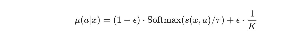
This policy works as follows:

• With probability (1−ϵ), it chooses an arm based on a Softmax distribution of the Matrix Factorization scores, where the temperature τ=0.7 controls randomness.

• With probability ϵ=0.05, it ignores the scores and chooses a movie uniformly at random from the K candidates. This guarantees that every arm has a non-zero chance of being selected, which is critical for unbiased offline learning.

• For each action taken, we record the probability μ(a∣x), known as the propensity score, which is essential for the next steps.

3. Training the Reward Model (Q^​)

Our logs only tell us the reward for the action we took, but it's helpful to estimate the potential rewards for all other arms. We train a reward model, Q^​(x,a), to predict the probability of a click for any given context-action pair.

• Model: The model is a Multi-Layer Perceptron (MLP) with one hidden layer of 128 units and a ReLU activation function.

• Features: Its input is a rich feature vector combining the user's context vector with features of the specific movie, including its embedding, its genre vector, and the element-wise product of the user and movie embeddings.

• Training: We train this model for 5 epochs using the AdamW optimizer and a Binary Cross-Entropy loss function to predict the observed binary reward from our simulated logs.

4. Training the Bandit Policy (π_θ​)

This is where we train our new, smart contextual bandit policy, π_θ​(a∣x). The goal is to learn a policy that maximizes the total expected reward.

• Model: The policy network is also an MLP with a similar architecture to the reward model. It takes the feature vectors for all K candidate arms and outputs K logits, which are converted via a Softmax function into a probability distribution over the arms.

• Objective: We train the policy to maximize the Doubly-Robust (DR) estimator, which provides a low-variance and unbiased objective function for offline policy learning. The objective:

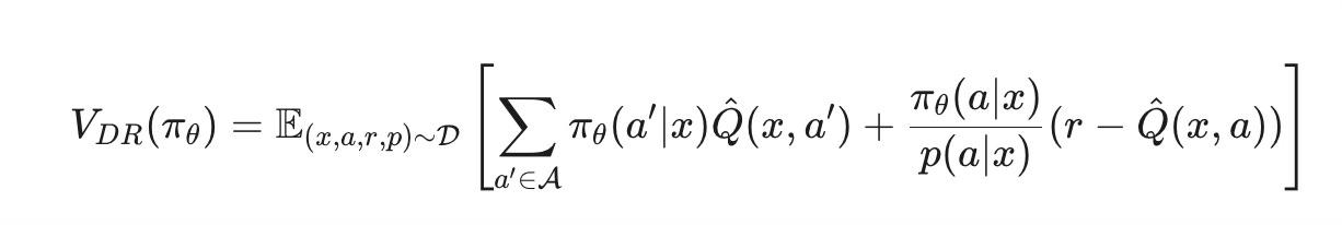
This formula looks complex, but it has two intuitive parts:

1. Direct Method term: ∑​πθ​(a′∣x)Q^​(x,a′). This uses our reward model Q^​ to estimate the value of our new policy directly. It has low variance but could be biased if Q^​ is inaccurate.

2. Importance Sampling term: This uses the real reward r and corrects for the difference between our new policy and the old logging policy using the propensity ratio​​. It then subtracts the reward model's prediction to correct for its own estimate. This term is unbiased but can have high variance.

By combining them, the DR estimator remains unbiased if either the reward model Q^​ or the propensity score p(a∣x) is correct, making it very robust. We train our policy to maximize this value.

The policy is trained for 8 epochs using the AdamW optimizer. To stabilize training, we use importance weight clipping (capping weights at 10.0) and add a small entropy bonus to the loss function to encourage the policy to maintain some exploration.

Evaluation and Results

How can we be sure our newly trained policy is any good without deploying it to live users? This is the challenge of Off-Policy Evaluation (OPE). We use our held-out test set of simulated logs to estimate what the click-through rate (CTR) of our new policy would have been. We use two common OPE metrics.

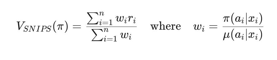
1. Self-Normalized Importance Sampling (SNIPS): This method re-weights the observed rewards from the test log based on how likely our new policy was to make the same choice compared to the original logging policy. The formula is:

   

   The normalization in the denominator helps stabilize the estimate.

2. Doubly Robust (DR) Estimator: We can also use the same DR formula from training for evaluation. It's often considered the gold standard for OPE due to its robustness.

Running our trained policy over the test log yields the following estimated CTRs:

• SNIPS CTR Estimate: 0.7952

• DR CTR Estimate: 0.1940

The significant difference between the two estimates highlights a common challenge in OPE. The SNIPS estimate is likely inflated due to high variance in the importance weights (wi​), which can happen when the new policy is very different from the logging policy. The DR estimate, which is stabilized by the reward model, is generally considered more reliable in such cases. The result suggests our new contextual bandit policy would achieve an impressive 19.4% click-through rate, demonstrating its ability to learn effective recommendation strategies from offline data.

Conclusion

In this post, we successfully built and evaluated a contextual bandit for recommendations from scratch. We started with raw historical data, learned meaningful user and item representations, and simulated a realistic interaction log. Using this log, we trained a new policy with the robust Doubly-Robust estimator and, finally, used Off-Policy Evaluation techniques to validate its performance.

This offline approach is a powerful and safe paradigm for developing modern, adaptive recommendation systems. It allows data scientists to iterate on and assess the impact of new policies, ensuring that only the most promising models are deployed into production. Contextual bandits represent a shift towards more intelligent, responsive, and ultimately more engaging user experiences.